


このブログでは、PatchTSTの使い方を例示します。まず、ElectricityデータセットでPatchTSTの予測能力を示します。次に、事前学習済みモデルを用いて電気変圧器(ETTh1)データセットでゼロショット予測を行い、PatchTSTの転移学習能力を示します。ゼロショット予測のパフォーマンスは、ターゲットドメインでのモデルのtestパフォーマンスを示し、ターゲットドメインでの学習は一切行いません。その後、ターゲットデータのtrain部分で事前学習済みモデルに対してlinear probingを行い、続いてfinetuningを行い、ターゲットデータのtest部分で予測パフォーマンスを検証します。
PatchTSTモデルは、Yuqi Nie、Nam H. Nguyen、Phanwadee Sinthong、Jayant Kalagnanamによって提案され、A Time Series is Worth 64 Words: Long-term Forecasting with TransformersとしてICLR 2023で発表されました。
PatchTSTの概要
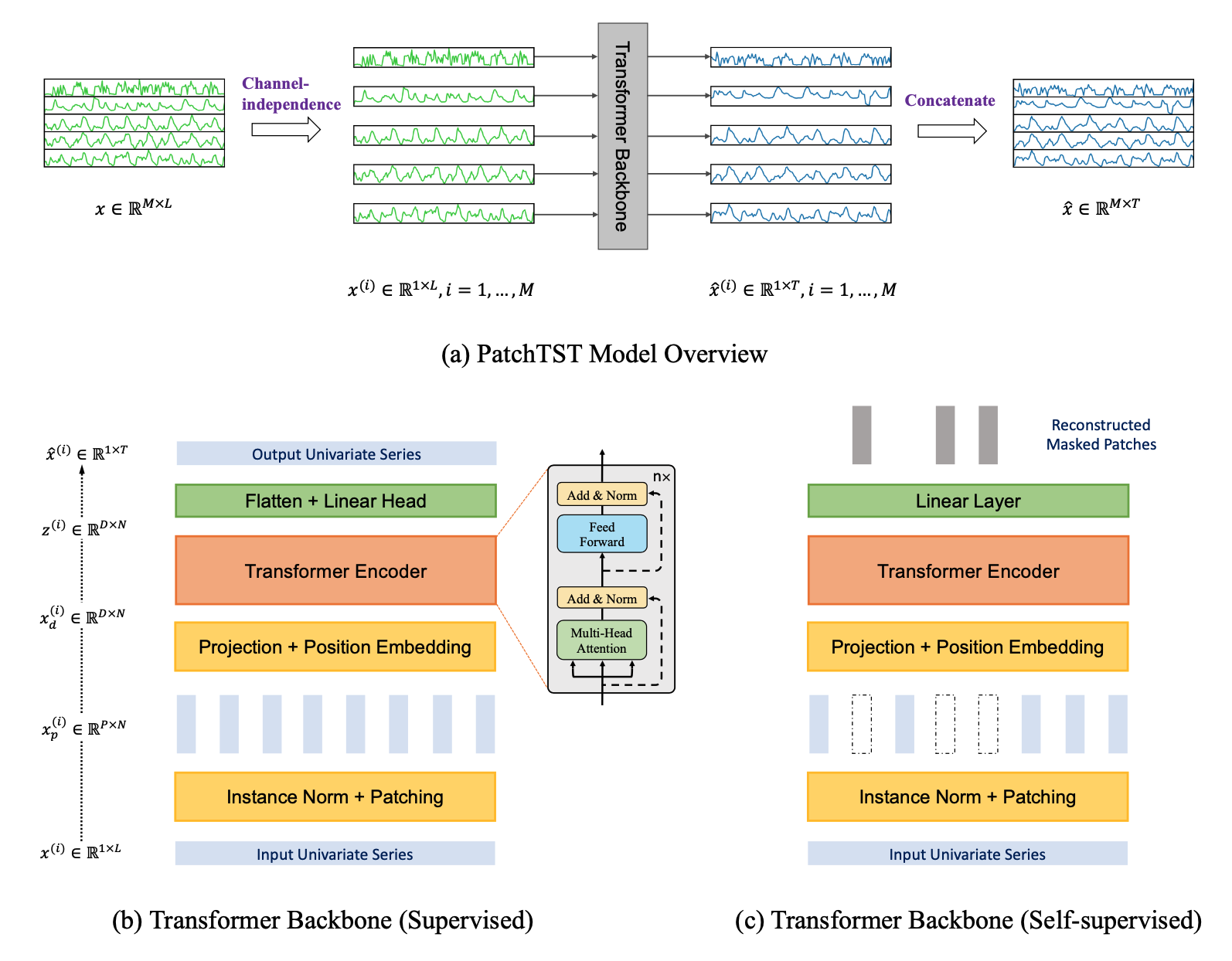
大まかに言うと、このモデルはバッチ内の個々の時系列を指定されたサイズのパッチにベクトル化し、その結果得られるベクトルのシーケンスをTransformerでエンコードし、適切なヘッドを介して予測長の予測を出力します。
このモデルは2つの主要なコンポーネントに基づいています:
- Transformerへの入力トークンとして機能するサブ系列レベルのパッチへの時系列のセグメンテーション;
- 各チャネルが単一の単変量時系列を含み、すべての系列で同じ埋め込みとTransformerの重みを共有するチャネル独立性、つまりグローバル単変量モデル。
パッチング設計には自然に3つの利点があります:
- 局所的な意味情報が埋め込みに保持される;
- 同じルックバックウィンドウにおいて、パッチ間のストライドによりアテンションマップの計算量とメモリ使用量が2次的に削減される;
- パッチ長(入力ベクトルサイズ)とコンテキスト長(シーケンス数)のトレードオフにより、より長い履歴に注意を向けることができる。
さらに、PatchTSTはマスク付き時系列事前学習と直接的な時系列予測をシームレスにサポートするモジュラー設計を備えています。
 |
|---|
| (a) PatchTSTモデルの概要。長さLLのMM個の時系列からなるバッチが、Transformerバックボーンを介して(バッチ次元に変形することで)独立に処理され、その結果得られたバッチが予測長TTのMM 系列に再変形される。各単変量系列は、ベクトルのパッチ化された集合を完全な予測長を出力するために使用する教師あり方式(b)、またはマスクされたパッチを予測する自己教師あり方式(c)で処理可能。 |
インストール
このデモでは、モデル用にHugging FaceのTransformersと、補助的なデータ前処理用にIBMのtsfmパッケージが必要です。
両方をインストールするには、tsfmリポジトリをクローンし、以下の手順に従います。
- IBM Time Series Foundation Modelリポジトリの公開版
tsfmをクローンします。pip install git+https://github.com/IBM/tsfm.git - Hugging Faceの
Transformersをインストールします。pip install transformers pythonターミナルで以下のコマンドでテストします。from transformers import PatchTSTConfig from tsfm_public.toolkit.dataset import ForecastDFDataset
Part 1: Electricityデータセットでの予測
ここでは、Electricityデータセット(https://github.com/zhouhaoyi/Informer2020から入手可能)でPatchTSTモデルを直接学習し、そのパフォーマンスを評価します。
# Standard
import os

# Third Party
from transformers import (
    EarlyStoppingCallback,
    PatchTSTConfig,
    PatchTSTForPrediction,
    Trainer,
    TrainingArguments,
)
import numpy as np
import pandas as pd

# First Party
from tsfm_public.toolkit.dataset import ForecastDFDataset
from tsfm_public.toolkit.time_series_preprocessor import TimeSeriesPreprocessor
from tsfm_public.toolkit.util import select_by_index
シードの設定
from transformers import set_seed

set_seed(2023)
データセットの読み込みと準備
次のセルでは、アプリケーションに合わせて以下のパラメータを調整してください:
dataset_path: ローカルの.csvファイルへのパス、または対象データのcsvファイルへのWebアドレス。データはpandasで読み込まれるため、pd.read_csvでサポートされるものはすべてサポートされます:(https://pandas.pydata.org/pandas-docs/stable/reference/api/pandas.read_csv.html)。timestamp_column: タイムスタンプ情報を含む列名。該当する列がない場合はNoneを使用。id_columns: 異なる時系列のIDを指定する列名のリスト。ID列が存在しない場合は[]を使用。forecast_columns: モデル化する列のリストcontext_length: モデルへの入力として使用される履歴データの量。context_lengthに等しい長さの入力時系列データのウィンドウが入力データフレームから抽出されます。多時系列データセットの場合、コンテキストウィンドウは単一の時系列(単一のID)内に含まれるように作成されます。forecast_horizon: 将来予測するタイムスタンプの数。train_start_index、train_end_index: 読み込まれたデータ内で学習データを区切る開始インデックスと終了インデックス。valid_start_index、eval_end_index: 読み込まれたデータ内で検証データを区切る開始インデックスと終了インデックス。test_start_index、eval_end_index: 読み込まれたデータ内でテストデータを区切る開始インデックスと終了インデックス。patch_length:PatchTSTモデルのパッチ長。context_lengthを均等に分割する値を選ぶことを推奨。num_workers: PyTorchデータローダーのCPUワーカー数。batch_size: バッチサイズ。
データはまずPandasデータフレームに読み込まれ、学習、検証、テストの各部分に分割されます。その後、Pandasデータフレームは学習に必要な適切なPyTorchデータセットに変換されます。
# The ECL data is available from https://github.com/zhouhaoyi/Informer2020?tab=readme-ov-file#data
dataset_path = "~/data/ECL.csv"
timestamp_column = "date"
id_columns = []

context_length = 512
forecast_horizon = 96
patch_length = 16
num_workers = 16  # Reduce this if you have low number of CPU cores
batch_size = 64  # Adjust according to GPU memory
data = pd.read_csv(
    dataset_path,
    parse_dates=[timestamp_column],
)
forecast_columns = list(data.columns[1:])

# get split
num_train = int(len(data) * 0.7)
num_test = int(len(data) * 0.2)
num_valid = len(data) - num_train - num_test
border1s = [
    0,
    num_train - context_length,
    len(data) - num_test - context_length,
]
border2s = [num_train, num_train + num_valid, len(data)]

train_start_index = border1s[0]  # None indicates beginning of dataset
train_end_index = border2s[0]

# we shift the start of the evaluation period back by context length so that
# the first evaluation timestamp is immediately following the training data
valid_start_index = border1s[1]
valid_end_index = border2s[1]

test_start_index = border1s[2]
test_end_index = border2s[2]

train_data = select_by_index(
    data,
    id_columns=id_columns,
    start_index=train_start_index,
    end_index=train_end_index,
)
valid_data = select_by_index(
    data,
    id_columns=id_columns,
    start_index=valid_start_index,
    end_index=valid_end_index,
)
test_data = select_by_index(
    data,
    id_columns=id_columns,
    start_index=test_start_index,
    end_index=test_end_index,
)

time_series_preprocessor = TimeSeriesPreprocessor(
    timestamp_column=timestamp_column,
    id_columns=id_columns,
    input_columns=forecast_columns,
    output_columns=forecast_columns,
    scaling=True,
)
time_series_preprocessor = time_series_preprocessor.train(train_data)
train_dataset = ForecastDFDataset(
    time_series_preprocessor.preprocess(train_data),
    id_columns=id_columns,
    timestamp_column="date",
    input_columns=forecast_columns,
    output_columns=forecast_columns,
    context_length=context_length,
    prediction_length=forecast_horizon,
)
valid_dataset = ForecastDFDataset(
    time_series_preprocessor.preprocess(valid_data),
    id_columns=id_columns,
    timestamp_column="date",
    input_columns=forecast_columns,
    output_columns=forecast_columns,
    context_length=context_length,
    prediction_length=forecast_horizon,
)
test_dataset = ForecastDFDataset(
    time_series_preprocessor.preprocess(test_data),
    id_columns=id_columns,
    timestamp_column="date",
    input_columns=forecast_columns,
    output_columns=forecast_columns,
    context_length=context_length,
    prediction_length=forecast_horizon,
)
PatchTSTモデルの設定
次に、設定を用いてランダムに初期化されたPatchTSTモデルをインスタンス化します。以下の設定は、アーキテクチャに関連するさまざまなハイパーパラメータを制御します。
num_input_channels: 時系列データの入力チャネル(または次元)の数。これは自動的に予測列の数に設定されます。context_length: 上記で説明した、モデルへの入力として使用される履歴データの量。patch_length: コンテキストウィンドウ(長さはcontext_length)から抽出されたパッチの長さ。patch_stride: コンテキストウィンドウからパッチを抽出する際に使用されるストライド。random_mask_ratio: モデルの事前学習のために完全にマスクされる入力パッチの割合。d_model: Transformerレイヤーの次元。num_attention_heads: Transformerエンコーダーの各アテンションレイヤーのアテンションヘッド数。num_hidden_layers: エンコーダーレイヤーの数。ffn_dim: エンコーダーの中間(しばしばフィードフォワードと呼ばれる)レイヤーの次元。dropout: エンコーダーの全結合レイヤーすべてのドロップアウト確率。head_dropout: モデルのヘッドで使用されるドロップアウト確率。pooling_type: 埋め込みのプーリング。"mean"、"max"、Noneがサポートされます。channel_attention: Transformer内でチャネルアテンションブロックを有効にし、チャネル同士が互いにアテンションできるようにする。scaling: 入力ターゲットを"mean"スケーラー、"std"スケーラー、またはNoneの場合はスケーラーなしでスケーリングするかどうか。Trueの場合、スケーラーは"mean"に設定されます。loss:distribution_outputヘッドに対応するモデルの損失関数。パラメトリック分布の場合は負の対数尤度("nll")、点推定の場合は平均二乗誤差"mse"。pre_norm: pre_normがTrueに設定されている場合、自己アテンションの前に正規化が適用されます。それ以外の場合、正規化は残差ブロックの後に適用されます。norm_type: 各Transformerレイヤーでの正規化。"BatchNorm"または"LayerNorm"が可能です。
パラメータの詳細については、ドキュメントを参照してください。
config = PatchTSTConfig(
    num_input_channels=len(forecast_columns),
    context_length=context_length,
    patch_length=patch_length,
    patch_stride=patch_length,
    prediction_length=forecast_horizon,
    random_mask_ratio=0.4,
    d_model=128,
    num_attention_heads=16,
    num_hidden_layers=3,
    ffn_dim=256,
    dropout=0.2,
    head_dropout=0.2,
    pooling_type=None,
    channel_attention=False,
    scaling="std",
    loss="mse",
    pre_norm=True,
    norm_type="batchnorm",
)
model = PatchTSTForPrediction(config)
モデルの学習
次に、Hugging FaceのTrainerクラスを活用して、直接予測戦略に基づいてモデルを学習できます。まず、エポック数、学習率などの学習に関するさまざまなハイパーパラメータをリストアップしたTrainingArgumentsを定義します。
training_args = TrainingArguments(
    output_dir="./checkpoint/patchtst/electricity/pretrain/output/",
    overwrite_output_dir=True,
    # learning_rate=0.001,
    num_train_epochs=100,
    do_eval=True,
    evaluation_strategy="epoch",
    per_device_train_batch_size=batch_size,
    per_device_eval_batch_size=batch_size,
    dataloader_num_workers=num_workers,
    save_strategy="epoch",
    logging_strategy="epoch",
    save_total_limit=3,
    logging_dir="./checkpoint/patchtst/electricity/pretrain/logs/",  # Make sure to specify a logging directory
    load_best_model_at_end=True,  # Load the best model when training ends
    metric_for_best_model="eval_loss",  # Metric to monitor for early stopping
    greater_is_better=False,  # For loss
    label_names=["future_values"],
)

# Create the early stopping callback
early_stopping_callback = EarlyStoppingCallback(
    early_stopping_patience=10,  # Number of epochs with no improvement after which to stop
    early_stopping_threshold=0.0001,  # Minimum improvement required to consider as improvement
)

# define trainer
trainer = Trainer(
    model=model,
    args=training_args,
    train_dataset=train_dataset,
    eval_dataset=valid_dataset,
    callbacks=[early_stopping_callback],
    # compute_metrics=compute_metrics,
)

# pretrain
trainer.train()
| エポック | 学習損失 | 検証損失 |
|---|---|---|
| 1 | 0.455400 | 0.215057 |
| 2 | 0.241000 | 0.179336 |
| 3 | 0.209000 | 0.158522 |
| ... | ... | ... |
| 83 | 0.128000 | 0.111213 |
ソースドメインのテストセットでモデルを評価
次に、trainer.evaluate()を活用してテストメトリクスを計算できます。これはこのタスクで判断するターゲットメトリクスではありませんが、事前学習済みモデルが適切に学習されたかどうかの妥当なチェックを提供します。
PatchTSTの学習損失と評価損失は平均二乗誤差(MSE)損失であることに注意してください。したがって、以下の評価実験ではMSEメトリクスを別途計算しません。
results = trainer.evaluate(test_dataset)
print("Test result:")
print(results)

>>> Test result:
    {'eval_loss': 0.1316315233707428, 'eval_runtime': 5.8077, 'eval_samples_per_second': 889.332, 'eval_steps_per_second': 3.616, 'epoch': 83.0}
0.131のMSEは、元のPatchTST論文で報告されたElectricityデータセットの値に非常に近いです。
モデルの保存
save_dir = "patchtst/electricity/model/pretrain/"
os.makedirs(save_dir, exist_ok=True)
trainer.save_model(save_dir)
Part 2: ElectricityからETTh1への転移学習
このセクションでは、PatchTSTモデルの転移学習能力を示します。
Electricityデータセットで事前学習したモデルを使用して、ETTh1データセットでゼロショット予測を行います。
転移学習とは、まずsourceデータセットで予測タスクの事前学習を行い(上記ではElectricityデータセットで行いました)、次に事前学習済みモデルをtargetデータセットでゼロショット予測に使用することを意味します。ゼロショットとは、追加の学習を行わずにtargetドメインでのパフォーマンスをテストすることを意味します。事前学習で得た知識が異なるデータセットに転移できることを期待します。
その後、ターゲットデータのtrain分割で事前学習済みモデルに対してlinear probingを行い、続いてfinetuningを行い、ターゲットデータのtest分割で予測パフォーマンスを検証します。この例では、ソースデータセットはElectricityデータセット、ターゲットデータセットはETTh1です。
ETTh1データでの転移学習
すべての評価はETTh1データのtest部分で行われます。
ステップ1: electricity事前学習済みモデルを直接評価。これはゼロショットパフォーマンスです。
ステップ2: linear probingを行った後に評価。
ステップ3: 完全なfinetuningを行った後に評価。
ETThデータセットの読み込み
以下では、ETTh1データセットをPandasデータフレームとして読み込みます。次に、学習、検証、テスト用の3つの分割を作成します。その後、TimeSeriesPreprocessorクラスを活用して各分割をモデル用に準備します。
dataset = "ETTh1"
print(f"Loading target dataset: {dataset}")
dataset_path = f"https://raw.githubusercontent.com/zhouhaoyi/ETDataset/main/ETT-small/{dataset}.csv"
timestamp_column = "date"
id_columns = []
forecast_columns = ["HUFL", "HULL", "MUFL", "MULL", "LUFL", "LULL", "OT"]
train_start_index = None  # None indicates beginning of dataset
train_end_index = 12 * 30 * 24

# we shift the start of the evaluation period back by context length so that
# the first evaluation timestamp is immediately following the training data
valid_start_index = 12 * 30 * 24 - context_length
valid_end_index = 12 * 30 * 24 + 4 * 30 * 24

test_start_index = 12 * 30 * 24 + 4 * 30 * 24 - context_length
test_end_index = 12 * 30 * 24 + 8 * 30 * 24

>>> Loading target dataset: ETTh1
data = pd.read_csv(
    dataset_path,
    parse_dates=[timestamp_column],
)

train_data = select_by_index(
    data,
    id_columns=id_columns,
    start_index=train_start_index,
    end_index=train_end_index,
)
valid_data = select_by_index(
    data,
    id_columns=id_columns,
    start_index=valid_start_index,
    end_index=valid_end_index,
)
test_data = select_by_index(
    data,
    id_columns=id_columns,
    start_index=test_start_index,
    end_index=test_end_index,
)

time_series_preprocessor = TimeSeriesPreprocessor(
    timestamp_column=timestamp_column,
    id_columns=id_columns,
    input_columns=forecast_columns,
    output_columns=forecast_columns,
    scaling=True,
)
time_series_preprocessor = time_series_preprocessor.train(train_data)
train_dataset = ForecastDFDataset(
    time_series_preprocessor.preprocess(train_data),
    id_columns=id_columns,
    input_columns=forecast_columns,
    output_columns=forecast_columns,
    context_length=context_length,
    prediction_length=forecast_horizon,
)
valid_dataset = ForecastDFDataset(
    time_series_preprocessor.preprocess(valid_data),
    id_columns=id_columns,
    input_columns=forecast_columns,
    output_columns=forecast_columns,
    context_length=context_length,
    prediction_length=forecast_horizon,
)
test_dataset = ForecastDFDataset(
    time_series_preprocessor.preprocess(test_data),
    id_columns=id_columns,
    input_columns=forecast_columns,
    output_columns=forecast_columns,
    context_length=context_length,
    prediction_length=forecast_horizon,
)
ETTHでのゼロショット予測
即座に予測パフォーマンスをテストするため、上記で事前学習したモデルを読み込みます。
finetune_forecast_model = PatchTSTForPrediction.from_pretrained(
    "patchtst/electricity/model/pretrain/",
    num_input_channels=len(forecast_columns),
    head_dropout=0.7,
)
finetune_forecast_args = TrainingArguments(
    output_dir="./checkpoint/patchtst/transfer/finetune/output/",
    overwrite_output_dir=True,
    learning_rate=0.0001,
    num_train_epochs=100,
    do_eval=True,
    evaluation_strategy="epoch",
    per_device_train_batch_size=batch_size,
    per_device_eval_batch_size=batch_size,
    dataloader_num_workers=num_workers,
    report_to="tensorboard",
    save_strategy="epoch",
    logging_strategy="epoch",
    save_total_limit=3,
    logging_dir="./checkpoint/patchtst/transfer/finetune/logs/",  # Make sure to specify a logging directory
    load_best_model_at_end=True,  # Load the best model when training ends
    metric_for_best_model="eval_loss",  # Metric to monitor for early stopping
    greater_is_better=False,  # For loss
    label_names=["future_values"],
)

# Create a new early stopping callback with faster convergence properties
early_stopping_callback = EarlyStoppingCallback(
    early_stopping_patience=10,  # Number of epochs with no improvement after which to stop
    early_stopping_threshold=0.001,  # Minimum improvement required to consider as improvement
)

finetune_forecast_trainer = Trainer(
    model=finetune_forecast_model,
    args=finetune_forecast_args,
    train_dataset=train_dataset,
    eval_dataset=valid_dataset,
    callbacks=[early_stopping_callback],
)

print("\n\nDoing zero-shot forecasting on target data")
result = finetune_forecast_trainer.evaluate(test_dataset)
print("Target data zero-shot forecasting result:")
print(result)

>>> Doing zero-shot forecasting on target data

    Target data zero-shot forecasting result:
    {'eval_loss': 0.3728715181350708, 'eval_runtime': 0.95, 'eval_samples_per_second': 2931.527, 'eval_steps_per_second': 11.579}
ご覧のとおり、ゼロショット予測アプローチにより、MSE 0.370が得られ、これは元のPatchTST論文で報告された最先端の結果に近い値です。
次に、凍結された事前学習済みモデルの上に線形層を学習するlinear probingを行うことで、どの程度改善できるかを見てみましょう。linear probingは、事前学習済みモデルの特徴量のパフォーマンスをテストするためによく行われます。
ETTh1でのlinear probing
ターゲットデータのtrain部分でquick linear probingを行い、testパフォーマンスの改善の可能性を確認できます。
# Freeze the backbone of the model
for param in finetune_forecast_trainer.model.model.parameters():
    param.requires_grad = False

print("\n\nLinear probing on the target data")
finetune_forecast_trainer.train()
print("Evaluating")
result = finetune_forecast_trainer.evaluate(test_dataset)
print("Target data head/linear probing result:")
print(result)

>>> Linear probing on the target data
| エポック | 学習損失 | 検証損失 |
|---|---|---|
| 1 | 0.384600 | 0.688319 |
| 2 | 0.374200 | 0.678159 |
| 3 | 0.368400 | 0.667633 |
| ... | ... | ... |
>>> Evaluating

    Target data head/linear probing result:
    {'eval_loss': 0.35652095079421997, 'eval_runtime': 1.1537, 'eval_samples_per_second': 2413.986, 'eval_steps_per_second': 9.535, 'epoch': 18.0}
ご覧のとおり、凍結されたバックボーンの上に単純な線形層を学習するだけで、MSEが0.370から0.357に減少し、元々報告された結果を上回りました!
save_dir = f"patchtst/electricity/model/transfer/{dataset}/model/linear_probe/"
os.makedirs(save_dir, exist_ok=True)
finetune_forecast_trainer.save_model(save_dir)

save_dir = f"patchtst/electricity/model/transfer/{dataset}/preprocessor/"
os.makedirs(save_dir, exist_ok=True)
time_series_preprocessor = time_series_preprocessor.save_pretrained(save_dir)
最後に、モデルの完全なfine-tuneを行うことで、さらに改善が得られるかどうかを見てみましょう。
ETTh1での完全なfine-tune
ターゲットデータのtrain部分でモデルの完全なfine-tune(上記のように最後の線形層をprobingするのではなく)を行い、testパフォーマンスの改善の可能性を確認できます。コードは上記のlinear probingタスクと似ていますが、パラメータを凍結しない点が異なります。
# Reload the model
finetune_forecast_model = PatchTSTForPrediction.from_pretrained(
    "patchtst/electricity/model/pretrain/",
    num_input_channels=len(forecast_columns),
    dropout=0.7,
    head_dropout=0.7,
)
finetune_forecast_trainer = Trainer(
    model=finetune_forecast_model,
    args=finetune_forecast_args,
    train_dataset=train_dataset,
    eval_dataset=valid_dataset,
    callbacks=[early_stopping_callback],
)
print("\n\nFinetuning on the target data")
finetune_forecast_trainer.train()
print("Evaluating")
result = finetune_forecast_trainer.evaluate(test_dataset)
print("Target data full finetune result:")
print(result)

>>> Finetuning on the target data
| エポック | 学習損失 | 検証損失 |
|---|---|---|
| 1 | 0.348600 | 0.709915 |
| 2 | 0.328800 | 0.706537 |
| 3 | 0.319700 | 0.741892 |
| ... | ... | ... |
>>> Evaluating

    Target data full finetune result:
    {'eval_loss': 0.354232519865036, 'eval_runtime': 1.0715, 'eval_samples_per_second': 2599.18, 'eval_steps_per_second': 10.266, 'epoch': 12.0}
この場合、ETTh1データセットでは完全なfine-tuningによる改善はわずかでした。他のデータセットでは、より大きな改善が見られる可能性があります。いずれにせよ、モデルを保存しておきましょう。
save_dir = f"patchtst/electricity/model/transfer/{dataset}/model/fine_tuning/"
os.makedirs(save_dir, exist_ok=True)
finetune_forecast_trainer.save_model(save_dir)
まとめ
このブログでは、予測と転移学習に関連するタスクでPatchTSTを学習するためのステップバイステップガイドを提示し、さまざまなfine-tuningアプローチを示しました。予測ユースケースでのPatchTST HFモデルの容易な統合を促進することを目的としており、このコンテンツがPatchTSTの採用を加速させるための有用なリソースとなることを願っています。ブログをご覧いただきありがとうございました。この情報が皆様のプロジェクトに役立つことを願っています。
0 Comments
Log in to join the conversation.No comments yet. Be the first to share your thoughts.