


The only Python IDE you need.

This is a guest post from Naa Ashiorkor, a data scientist and tech community builder.
Building intelligent systems that can see, hear, understand language, and make decisions was previously the domain of specialized researchers with massive computing resources only – today, deep learning has made this accessible to developers and data scientists across the world, bringing the ability to build, train, and deploy AI models within reach.
This accessibility can be credited to deep learning frameworks, and one such framework is PyTorch, which has rapidly become the prevailing choice across both research and industry. PyTorch is an open-source deep learning framework built in Python and designed to make building neural networks intuitive.
Curious about how neural networks actually learn? In this tutorial, you’ll build your first PyTorch model using the MNIST dataset in PyCharm and see it recognize handwritten digits in real time. Along the way, you’ll get familiar with tensors and understand the core workflow behind building deep learning models.
What is PyTorch?
PyTorch traces its roots to Torch, a scientific computing framework that used Lua; in 2016, researchers at Facebook’s AI Research Lab (FAIR), now Meta AI, reinvented it for Python, creating PyTorch, which is today a Linux Foundation community project.
By 2024, PyTorch had established itself as the most popular deep learning framework, with a 63% adoption rate in the model training space, used in over 70% of AI research implementations. In 2025, the PyTorch Foundation’s ecosystem grew to include large-scale projects such as vLLM, DeepSpeed, and Ray, all of which are governed independently.
The annual PyTorch Conference attracted more than 3,400 attendees and gained 16 new industry members, including Snowflake, Dell Technologies, and Qualcomm. Also, it is trusted in production by organizations such as Meta, Microsoft, OpenAI, and Tesla. For developers and data scientists looking to enter deep learning, PyTorch remains the most practical and widely supported starting point available today.
PyTorch was built on two foundations: GPU-accelerated tensor computation as a more powerful alternative to NumPy and an automatic differentiation engine for training neural networks.
From these foundations, PyTorch has grown into one of the most fully featured deep learning frameworks available. Its core features include:
- Dynamic computation graphs (define-by-run): As code executes, PyTorch builds computation graphs. These are maps of every mathematical operation your model performs: things like multiplying inputs by weights, adding biases, and applying activation functions. PyTorch needs to track these because training requires working backwards through all of those steps to calculate how much each weight contributed to the model’s error, so it knows how to adjust them to improve. Computation graphs allow the model structure to be modified during runtime and facilitate debugging using standard Python tools, making PyTorch ideal for research and experimentation.
- Pythonic and intuitive interface: PyTorch code is Pythonic, which reduces the learning curve. It uses standard Python control flow and clean, readable syntax, and it integrates well with Pythonic libraries.
- Strong GPU acceleration: PyTorch has seamless support for GPUs using CUDA. There is easy device switching and efficient tensor computations on GPUs. It also supports multi-GPU training.
- Autograd (automatic differentiation): There is a built-in autograd engine that automatically computes gradients. It tracks operations on tensors and enables backpropagation with minimal code.
- Rich neural network library: PyTorch provides a comprehensive module for building models. There are prebuilt layers, loss functions, activation functions, and a modular design for custom architectures.
- Extensive ecosystem: PyTorch is not just a framework – it is an ecosystem. There is a wide array of tools, even beyond the AI-specific libraries. Hence, an entire AI project can be managed under the Python umbrella from data collection to deployment.
- Model deployment support: PyTorch supports deploying models from research to production, with support for both mobile and edge deployments. What’s more, it also has TorchScript for optimized execution and ONNX export for interoperability.
- Broad community and industry adoption: PyTorch is backed by Meta, and it has a large and active community. Due to Python being one of the largest programming communities worldwide, PyTorch users benefit from shared knowledge, resources, and tools. There is extensive documentation and tutorials, and it is widely used in academia and industry.
For a broader perspective on how PyTorch and TensorFlow differ, and when to choose each, check out this blog post.
Why use PyTorch for deep learning projects?
PyTorch is at the core of the current deep learning ecosystem. In recent years, it has been the framework behind some of the most influential AI models, such as Meta’s Llama, OpenAI’s early GPT models, and Stable Diffusion. Today, it is a popular choice for AI research worldwide.
With a 63% adoption rate, PyTorch is the industry leader in model training, according to the Linux Foundation’s Shaping the Future Generative AI report. In academia, it is highly used in research paper implementations. It is preferred for research and development because of its intuitive design, which allows for easy experimentation and iteration.
Hence, researchers can develop novel architectures and test ideas simultaneously. PyTorch powers 85% of deep learning papers presented at top AI conferences.
PyTorch is a framework of choice due to its advantages:
- Debugging with PyTorch is straightforward and natural since it runs as ordinary Python. Due to its dynamic graphing and real-time execution, developers can test and make changes to models using standard Python tools like print statements and debuggers – no special setups or workarounds are required. This sets PyTorch apart significantly from static-graph frameworks, where errors mostly emerge at runtime, and it can be challenging to trace them back to their source.
- PyTorch is flexible due to its dynamic computation graph and intuitive API, so it is ideal for experimentation and rapid iteration.
- PyTorch has a thriving community. According to the PyTorch 2024 year in review, there were contributions from more than 3,500 individuals and 3,000 organizations in a single year, and its tooling ecosystem grew by over 25%. The community has built up a huge library of tutorials, pre-trained models, and extensions. In particular, Hugging Face’s Transformers library, built directly on top of PyTorch, is now the standard toolkit for NLP research and development.
Understanding PyTorch tensors
Understanding PyTorch requires an understanding of tensors. Every input, output, and model weight in PyTorch lives inside a tensor. Hence, tensors are not just a data format; they are the medium through which all computation flows.
Tensors are the core data structure in PyTorch. They are like n-dimensional arrays and matrices, but unlike regular arrays, tensors can be used on hardware accelerators like GPUs. Think of tensors as an extension of numbers we are already familiar with. A single number is a zero-dimensional tensor, a list of numbers is a one-dimensional tensor, and a table of numbers is a two-dimensional tensor. From there, you can add more dimensions to represent complex data like images, videos, or audio.
Neural networks accept tensors as input and generate tensors as output – even the parameters of a neural network, its weights and biases, are stored as tensors. For a visual explanation, you can watch a beginner-friendly video on tensors and deep learning:
Tensors are similar to NumPy arrays but can also run on GPUs or other hardware accelerators. Often, tensors and NumPy arrays can share the same underlying memory, meaning that data doesn’t need to be copied.
The main difference is what happens when the calculation gets serious. NumPy is for scientific computing on a CPU. PyTorch tensors can be moved and processed on GPUs in one line of code, allowing for massive parallel computation and providing significant speedups for the types of matrix multiplication common in deep learning.
This enables the kind of processing that makes training large neural networks possible.
There are basic operations with PyTorch tensors that are essential. You can view the full implementation in this GitHub repository.
Creating a tensor
The first thing you need to know is how to create a tensor. PyTorch gives you several ways depending on what your data looks like – you can build a tensor from an existing list, initialize one filled with zeros or ones as a placeholder, or generate one with random values as a starting point for a model’s weights.
import torch

# From a list
x = torch.tensor([1.0, 2.0, 3.0])

# Filled with zeros or ones
zeros = torch.zeros(3, 3)
ones = torch.ones(3, 3)

# Random values
rand = torch.rand(3, 3)

print(x)
print(zeros)
print(ones)
print(rand)
This code snippet demonstrates different ways to create tensors in PyTorch. A tensor is created from a Python list, alongside tensors filled with zeros and ones, and a tensor containing randomly generated values. The output displays the resulting tensor structures and values, illustrating common methods used to initialize tensors for deep learning workflows.
Basic arithmetic
Tensor arithmetic works element-wise, meaning PyTorch applies the operation across every value in the tensor simultaneously rather than looping through one by one. This is what makes tensors so fast – and it is also what makes GPU acceleration so powerful, since GPUs are specifically designed to run thousands of these operations in parallel.
a = torch.tensor([1.0, 2.0, 3.0])
b = torch.tensor([4.0, 5.0, 6.0])

print(a + b)
print(a * b)
print(a.sum())
print(a.mean())
This code snippet demonstrates common mathematical operations on PyTorch tensors. Two tensors are added and multiplied element-wise, while functions such as sum() and mean() are used to compute the total and average values of the tensor elements. The output displays the results of these operations, highlighting how PyTorch efficiently performs numerical computations on tensor data.
Reshaping
In deep learning, you will constantly need to reshape tensors – for example, flattening a 2D image into a 1D vector before passing it into a fully connected layer or reorganizing a batch of data to match what a model expects as input. PyTorch makes this straightforward with reshape(), which rearranges the data into a new shape without changing the underlying values.
x = torch.ones(6)
x_reshaped = x.reshape(2, 3)
print(x_reshaped.shape)
This code snippet demonstrates how to change the shape of a tensor using the reshape() function. A one-dimensional tensor of ones containing six elements is reshaped into a 2×3 tensor. The output shows the updated tensor structure, confirming that the data has been reorganized without altering its values.
Moving to GPU
By default, tensors are created on the CPU, but moving them to a GPU – where matrix operations can run orders of magnitude faster – takes just one line. This allows the same code to run on both GPU-equipped machines and machines that only have a CPU. It is good practice to check whether a GPU is available.
if torch.cuda.is_available():
   x = x.to("cuda")
This code checks whether a CUDA-enabled GPU is available using torch.cuda.is_available(). If a GPU is available, the tensor x is moved from the CPU to the GPU using .to("cuda"). This enables faster computation by leveraging GPU acceleration, which is especially useful for large-scale deep learning tasks.
Converting to and from NumPy
PyTorch and NumPy use nearly the same language, so switching between them is simple. Chances are you are already using NumPy somewhere in your pipeline – for loading data, preprocessing, or visualizing results.
PyTorch is designed to work alongside it seamlessly. You can convert between tensors and NumPy arrays in one line, and on the CPU, they even share the same memory, so there is no performance cost to switching between them.
import numpy as np

# Tensor to NumPy
tensor = torch.tensor([1.0, 2.0, 3.0])
numpy_array = tensor.numpy()

print("Original PyTorch tensor:")
print(tensor)

print("\nConverted to NumPy array:")
print(numpy_array)

# NumPy to Tensor
numpy_array = np.array([1.0, 2.0, 3.0])
tensor = torch.from_numpy(numpy_array)

print("\nOriginal NumPy array:")
print(numpy_array)

print("\nConverted to PyTorch tensor:")
print(tensor)
This snippet demonstrates interoperability between PyTorch and NumPy. A PyTorch tensor is first converted into a NumPy array using .numpy(), and then a NumPy array is converted back into a PyTorch tensor using torch.from_numpy(). The output shows that the values remain unchanged during the conversion process, highlighting seamless data sharing between the two libraries. This is particularly useful when integrating PyTorch models with NumPy-based preprocessing or analysis workflows.
Setting up PyTorch
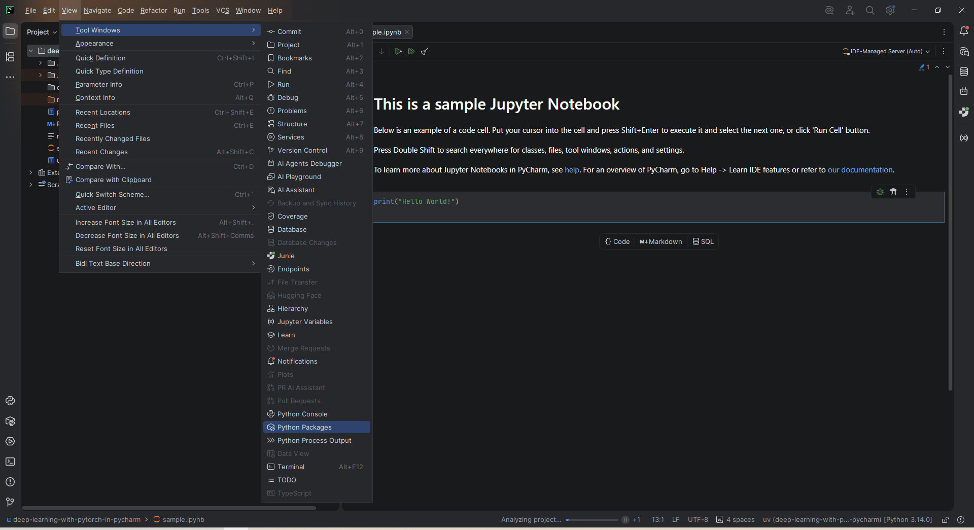
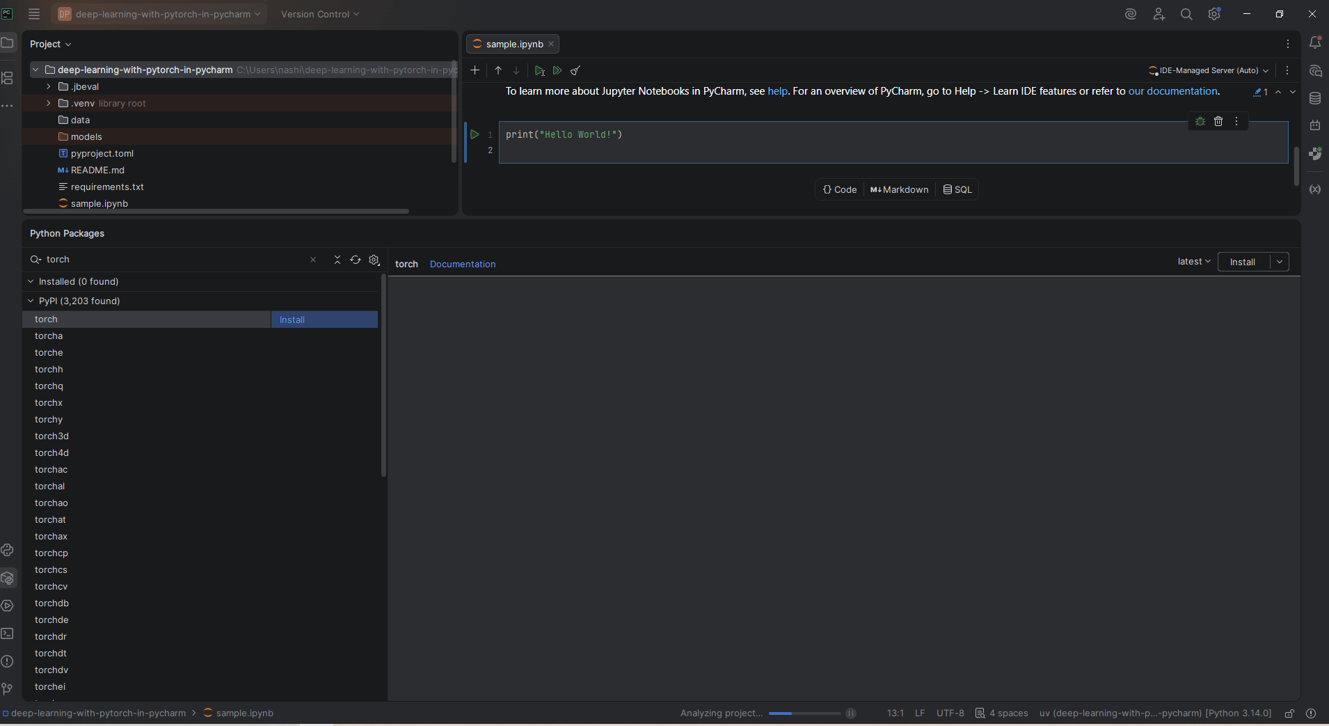
PyCharm streamlines deep learning setup by integrating directly with Python environments and package management tools. One of its key strengths is its seamless integration with Jupyter notebooks and optional Google Colab support, allowing you to switch between local and cloud-based computation effortlessly.
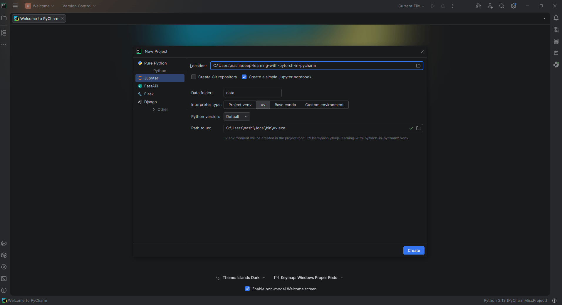
Before creating the project, it is important to install uv, a fast Python package and environment manager, locally. This enables PyCharm to create and manage project-specific environments using uv directly from the Python interpreter settings.
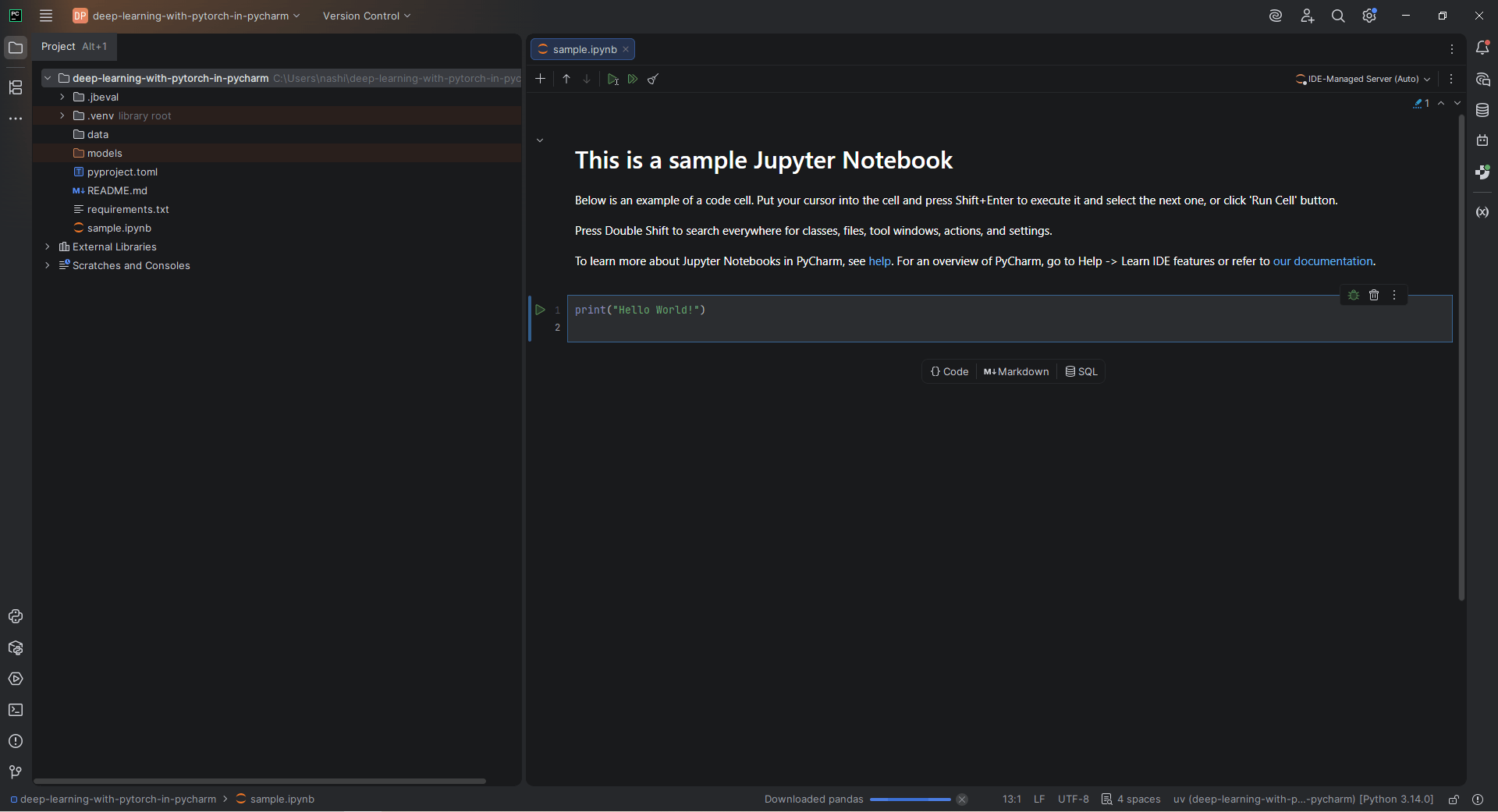
The setup process begins by creating a new project, where a project-specific Python environment is configured through the Python interpreter settings. During this step, a uv-managed environment and a Jupyter notebook are selected, too, enabling an interactive development environment from the beginning.
Version control can also be initialized using Git within this same window. For a detailed guide on creating and working with Jupyter notebooks in PyCharm, refer to the PyCharm documentation.
Using Conda as an alternative
If a Conda environment is preferred, PyCharm supports Conda directly through the Python interpreter settings. A Conda environment can be selected when setting up the project, and PyCharm will manage it automatically. Refer to the PyCharm documentation for Conda environments for more details on configuring them.
Once the Conda environment is active, install PyTorch using the terminal:
conda install pytorch torchvision torchaudio pytorch-cuda=12.1 -c pytorch -c nvidia
For PyTorch development, I recommend PyCharm because it provides excellent support for Python, intelligent coding assistance, debugging, version control, integrated database management, and seamless Docker integration. Specifically for data science, PyCharm supports Jupyter notebooks and key scientific and machine learning libraries and integrates with tools like the Hugging Face models library, Anaconda, and Databricks.
Additionally, it is particularly well-suited for PyTorch development because it understands the framework and includes features for layer-by-layer inspection of PyTorch tensors, which is essential when exploring data and building deep learning models.
Beyond tensors, PyCharm allows you to set breakpoints in training loops, inspect tensor values, and step through model forward passes using the integrated debugger – which works naturally with PyTorch’s dynamic computation graphs.
Building neural networks with PyTorch
A neural network is a system of connected layers that learns patterns from data by adjusting its internal weights through training. In PyTorch, all of these layers are contained within a single module called torch.nn . Think of it as your construction toolkit, which gives you everything you need to assemble a network without writing low-level mathematical operations from scratch.
torch.nn comes with a library of predefined layers, such as nn.Linear for fully connected layers, nn.Conv2d for convolutional layers, and nn.LSTM for recurrent layers. Hence, you can focus on designing your network rather than implementing the math behind each layer. It provides all the building blocks needed to build your own neural network.
Every module in PyTorch subclasses nn.Module. As a neural network is itself a module that consists of other modules (layers), this nested structure allows for easily building and managing complex architectures.
When you build a neural network in PyTorch, you create a Python class that inherits from nn.Module and implements two core methods:
__init__() –where you define your layers.forward() –where you define how data flows through those layers.
PyTorch’s autograd system automatically builds the computation graph based on the operations performed in the forward method, enabling automatic differentiation. The backward method, which handles gradient computation, typically does not need to be implemented manually. That means PyTorch handles the math behind gradient calculations, so you can focus on building.
Model building involves more than understanding the code. There are practicalities that need to be considered.
- Constant iteration. There is a very high probability that your first model will not perform well. That is normal because deep learning is an experimental process that involves adjusting layers, activation functions, and hyperparameters until the model improves.
- Simplicity first, then complexity. A two-layer feedforward network is always a good starting point. It is advisable to add complexity, such as additional layers and different architectures, when it is clear that the simple model is insufficient.
PyCharm makes model building easier thanks to its integrated debugger. You can set breakpoints inside your forward method, inspect tensor values at each layer, and add step-throughs of your model pass by pass, which drastically reduces the time it takes to identify and fix problems.
Build your first PyTorch handwritten digit classifier
In this section, you will build a simple neural network in PyTorch that can recognize handwritten digits from the MNIST dataset. You will work through the complete workflow, starting from raw image data; you will prepare and normalize the dataset, define a neural network, train it to recognize digits, and evaluate how well it performs on test data.
Along the way, you will explore key deep learning concepts such as tensors, layers, activation functions, loss functions, optimization, and training loops, while using PyCharm to inspect and understand what happens inside the training loop.
In deep learning, image classification is a foundational task, in which a model learns to assign a label to an image based on its visual content. In this example, we’ll use image classification on the MNIST database of handwritten digits, a classic benchmark in computer vision that consists of 28 x 28 grayscale images of handwritten digits from 0 to 9.
It is small and well-structured, and using it as an example gives us the opportunity to focus on understanding the core building blocks of deep learning. The aim is to build a neural network using PyTorch that can accurately recognize and classify these digits.
The complete source code for this project is available in the accompanying GitHub repository.

Preparing the data
Before training any model, the data needs to be loaded, cleaned, and formatted so PyTorch can work with it efficiently. PyTorch provides two classes that handle this:
Datasetdefines how individual samples are accessed and returned.DataLoadertakes aDatasetand handles how data is fed into the model during training, including batching, shuffling, and parallel loading.
As these components are configured, PyCharm helps streamline development through features such as code completion, automatic import suggestions, parameter hints, and quick documentation.
Hovering over PyTorch classes and functions shows usage information, and pressing Ctrl+Q opens detailed documentation directly within the IDE. Hence, it is easier to explore PyTorch APIs and correctly configure data loading and preprocessing steps without frequently switching to external documentation.
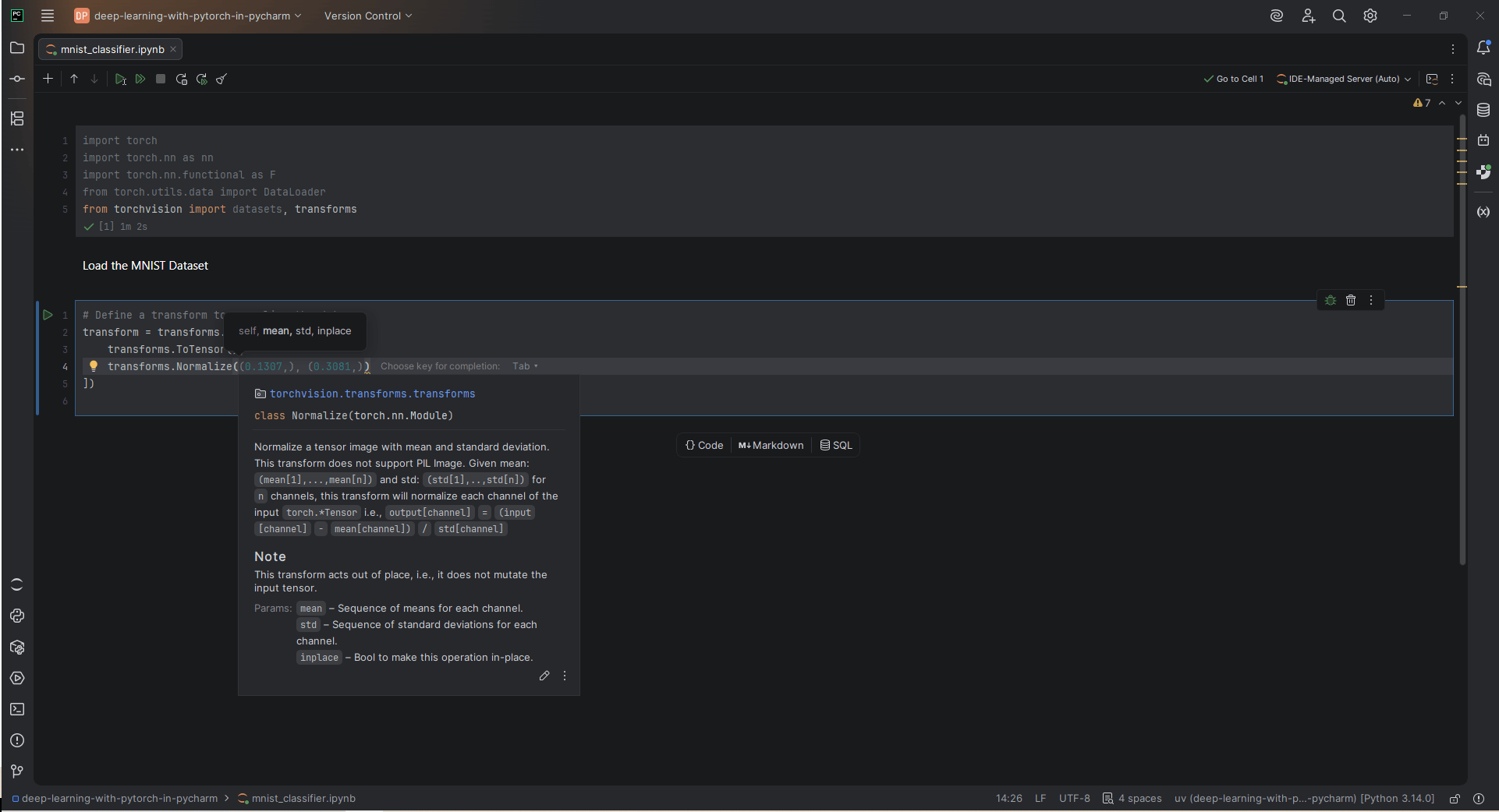
transforms.Normalize() is typed, PyCharm displays the function signature and parameter information directly in the editor, helping developers configure data preprocessing steps more efficiently without referring to external documentation. Loading and normalizing the data
Before training a neural network, the input data needs to be normalized so that the pixel values are scaled into a consistent range. This helps improve stability by keeping input values centered around zero and ensuring that gradients behave more predictably during optimization.
# Download and load the training data
train_data = datasets.MNIST(
   root='./data',
   train=True,
   download=True,
   transform=transform
)
The code snippet above downloads the MNIST dataset (if needed), loads the training images, and applies preprocessing so that the data is ready to be used in a neural network.
In this project, MNIST images are normalized as part of a preprocessing pipeline using PyTorch transforms:
transforms.ToTensor()converts images from pixel values (0–255) into floating-point tensors scaled to 0–1.transforms.Normalize((0.5,), (0.5,))then rescales these values to approximately -1 to 1, which helps stabilize training by keeping input values centered around zero and improving gradient behavior during optimization.
PyTorch also provides key data-loading parameters to control how training data is processed:
batch_size=64means the model processes 64 images at a time instead of the full dataset. This improves memory efficiency and makes training more stable by allowing gradient updates on mini-groups of data rather than individual samples or the entire dataset.shuffle=Truerandomizes the order of images each epoch, so the model does not memorize the sequence.download=Truemeans PyTorch fetches MNIST automatically on the first run, so you do not need to download anything manually.
Defining the model
After the data is ready the next step is to build the neural network that will learn from it. The goal of the model is to take an input image of a handwritten digit and predict which digit (0–9) it represents. Each MNIST image is 28×28 pixels. Since the model cannot directly interpret images the way humans do, we first flatten each image into a single vector of 784 values (28 x 28 = 784). This converts the 2D image into a format the model can process.
The input layer takes the 784 pixel values and passes them through fully connected layers. Each layer learns weighted combinations of features that become increasingly useful for distinguishing digits. While these representations are not explicitly interpretable, the network gradually learns patterns that help separate different classes.
To help the model learn effectively, we use an activation function called ReLU, which allows the network to capture non-linear patterns that are essential for understanding images.
class SimpleNetwork(nn.Module):
   def __init__(self):
       super(SimpleNetwork, self).__init__()
       self.fc1 = nn.Linear(784, 128)  # 28x28 = 784 input pixels
       self.fc2 = nn.Linear(128, 64)   # hidden layer
       self.fc3 = nn.Linear(64, 10)    # 10 outputs (digits 0-9)


   def forward(self, x):
       x = x.view(-1, 784)             # flatten the image
       x = F.relu(self.fc1(x))
       x = F.relu(self.fc2(x))
       x = self.fc3(x)
       return x


model = SimpleNetwork()
print(model)
When you run the code, PyTorch prints the structure of the model:
SimpleNetwork(
  (fc1): Linear(in_features=784, out_features=128, bias=True)
  (fc2): Linear(in_features=128, out_features=64, bias=True)
  (fc3): Linear(in_features=64, out_features=10, bias=True)
)
The output shows the structure of the neural network. Each Linear layer represents a fully connected layer in the model. The first layer transforms the 784 input pixels into 128 features, the second reduces them to 64 features, and the final layer outputs 10 values representing the digit classes (0–9). This confirms that the model has been correctly defined before training begins.
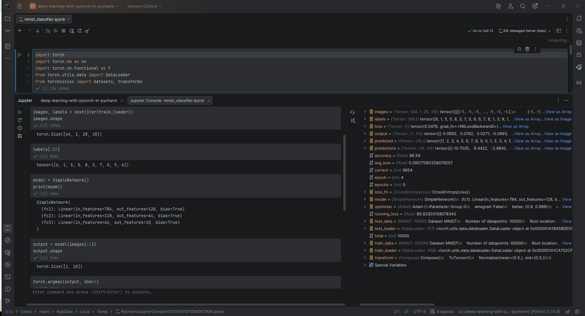
Using the Jupyter console to inspect data and validate the neural network
One of the features that makes PyCharm Pro especially useful for PyTorch development is the integrated Jupyter console. It connects directly to the running notebook kernel, allowing you to inspect tensors, explore datasets, test model outputs, and debug code interactively without adding temporary cells to the notebook. This streamlines the iterative workflow and makes it easier to validate code during model development.
To access the Jupyter console, first ensure that your Jupyter notebook is running. Then click Open Jupyter Console in the notebook toolbar at the top of the editor.
Additionally, PyCharm provides a Variables view that displays all active objects in the notebook kernel, allowing quick visual inspection of shapes, values, and types, and reducing the need for repeated print statements.
Together, these tools make it easier to inspect data and validate model behavior before training.
Training the model
Choosing a loss function and optimizer
Now that the model is defined, the next step is to train it so it can learn to recognize handwritten digits. During training, the model processes MNIST images, makes predictions, compares them to correct labels, and gradually improves its performance. To do this, we first need two key components: a loss function and an optimizer.
The loss function measures how far the model’s predictions are from the correct answers. In classification problems like MNIST (which has 10 classes, one for each digit), CrossEntropyLoss is used because it is designed for multi-class classification, and it not only penalizes incorrect predictions but also takes into account how confident the model is when it makes a mistake.
The optimizer is responsible for updating the model’s weights based on the loss. It determines how the model learns from its errors.
We also need to select an optimizer. Adaptive moment estimation (ADAM) and stochastic gradient descent (SGD) are two examples of these – they take the loss and adjust the model’s weights to do better next time.
The difference is how they do it. SGD updates model weights using a fixed learning rate applied to the computed gradients. ADAM extends this idea by adapting the learning rate for each parameter using estimates of past gradients, which often leads to faster and more stable convergence with less manual tuning. For this project, ADAM is the practical choice, with lr=0.001 as a safe default learning rate. SGD is worth exploring later when you want more control over the training process.
Implementing a training loop
The training loop is the core of the learning process. Each full pass through the training data is called an epoch. Training typically runs for multiple epochs so that the model can gradually improve its performance over time.
Each epoch is made up of smaller units called batches. Instead of processing the entire dataset at once, the model processes one batch at a time, which makes training more efficient and memory-friendly.
During each epoch, the model processes data in batches and repeats the same steps:
- Forward pass: The model makes predictions (logits).
- Loss computation: The model compares predictions with true labels.
- Backward pass: The model computes gradients of the loss.
- Weight update: The optimizer adjusts model parameters.
There are a few important implementation details to note when it comes to this section:
model.train()switches the model into training mode and must be called at the start of each epoch.optimizer.zero_grad()must be called beforeloss.backward()every iteration because, without it, PyTorch accumulates gradients from previous batches, which corrupts the updates. This is one of the most common beginner mistakes in PyTorch.loss.item()converts the loss tensor into a Python number for logging. This detaches it from the computation graph, ensuring it is not tracked for gradients.
The code below implements the training loop and prints the loss at the end of each epoch:
# Define loss function and optimizer
loss_fn = nn.CrossEntropyLoss()
optimizer = torch.optim.Adam(model.parameters(), lr=0.001)

# Training loop
epochs = 5

for epoch in range(epochs):
   model.train()
   running_loss = 0

   for images, labels in train_loader:
       # Forward pass
       predictions = model(images)
       loss = loss_fn(predictions, labels)

       # Backward pass
       optimizer.zero_grad()
       loss.backward()
       optimizer.step()

       running_loss += loss.item()

   avg_loss = running_loss / len(train_loader)
   print(f"Epoch {epoch+1}/5 — Loss: {avg_loss:.4f}")
The output below shows the model’s training progress over five epochs, with the loss steadily decreasing as learning improves.
Epoch 1/5 — Loss: 0.4014
Epoch 2/5 — Loss: 0.1937
Epoch 3/5 — Loss: 0.1364
Epoch 4/5 — Loss: 0.1116
Epoch 5/5 — Loss: 0.0957
Debugging the training process using the PyCharm debugger
While basic Python debugging is available in PyCharm, the PyCharm Pro subscription extends this capability by providing full support for debugging Jupyter notebooks and interactive machine learning workflows.
During model training, breakpoints can be set inside key stages of the training loop, such as the forward pass, allowing execution to pause while the notebook remains interactive. For the MNIST handwritten digit classification project developed in this tutorial, the breakpoint was placed on: predictions = model(images).
This marks the start of the forward pass, in which a batch of input images is passed through the neural network to generate predictions. Pausing execution immediately before this line makes it possible to inspect the input data before the model processes it and then examine the model’s outputs after stepping over the line. This provides a clear view of how data flows through the network during training.
In the PyCharm debugger, the Watches pane lets you monitor custom expressions whenever execution pauses at a breakpoint. Rather than repeatedly evaluating expressions manually, watches automatically refresh their values after each debugging step, making it easier to inspect tensors and verify intermediate results throughout the training process.
For this project, the following watches were added:
images.shape, to verify the dimensions of each input batch.labels.shape, to confirm that the batch of labels corresponds to the input images.predictions.shape, to verify that the network produces an output tensor of the expected shape after the forward pass.predictions.argmax(dim=1)[:5], to display the predicted digit for the first five images in the batch.
After stepping over the forward pass, these watches automatically update to display the model’s outputs. This makes it straightforward to verify that the input tensors have the expected dimensions, confirm that the network produces a prediction for each image in the batch, and inspect the predicted digit classes without modifying the source code.
The debugging workflow described in this section is demonstrated in this video:
Model evaluation
Training is done, but a low training loss does not necessarily mean your model is good. It might have simply memorized the training data. Evaluation on unseen test data tells you how well it actually generalizes. After five epochs of training, the model achieves a test accuracy of 96.87%, correctly classifying 9,687 out of 10,000 previously unseen digits.
This indicates that the model generalizes well to new data for a simple fully connected architecture without additional optimization techniques. It also demonstrates one of PyTorch’s biggest strengths in practice: You can go from raw data to a working, accurate model with relatively little code.
model.eval()
correct = 0
total = 0

with torch.no_grad():
   for images, labels in test_loader:
       predictions = model(images)
       _, predicted = torch.max(predictions, 1)
       total += labels.size(0)
       correct += (predicted == labels).sum().item()

accuracy = 100 * correct / total
print(f"Test Accuracy: {accuracy:.2f}%")
Advanced PyTorch techniques for deep learning
There are advanced PyTorch techniques that can be explored when you grasp building and training basic models. They can take your work further, for example by allowing you to train faster, scale larger, or move a model into production. Some of them include:
- GPU acceleration. One of the highest-impact changes you can make is moving your model and data to a GPU. Modern NVIDIA GPUs such as the A100, H100, and V100 are recommended to accelerate PyTorch with the greatest speedup. They offer exceptional performance, especially for features such as
torch.compile. - Distributed learning. When a single GPU is not enough – either because your model is too large or your dataset too vast – PyTorch’s
torch.distributedbackend lets you scale training across multiple GPUs or machines.DistributedDataParallel(DDP) enables distributed training across multiple GPUs or machines, significantly boosting compute power and reducing training time. When the capacity of a single GPU is exceeded by your model, DDP becomes essential and requires only a few additional lines of code to set up. - Model deployment. Training a model is just one key aspect; eventually, you need to deploy it to real users. TorchServe is a flexible and easy-to-use tool for serving Python models in production. It supports deploying models in either eager or graph mode using TorchScript, serving multiple models concurrently, versioning models for A/B testing, loading and unloading models dynamically, and monitoring detailed logs and customizable metrics.
These three techniques represent the natural progression of any advanced deep learning project. You start on a single machine, scale when needed, and ship when you are ready. They are worth exploring as your projects grow in ambition.
Summary and resources
In this tutorial, you went from understanding what PyTorch is to building and training a neural network that recognizes handwritten digits with over 96% accuracy. Also, we covered tensors, the torch.nn module, the training loop, and model evaluation, which are the core building blocks of every deep learning project built with PyTorch.
This is just the beginning. PyTorch’s real depth lies in what comes next – convolutional networks, transfer learning, and the vast Hugging Face ecosystem of pre-trained models, which run on a PyTorch backend, all built on the same foundations you learned here. Continue to experiment! Swap the optimizer, add a layer, and try a different dataset.
A great next step is to explore the official PyTorch tutorials, which cover everything from convolutional networks to deploying models in production. For a more structured learning path, the Zero to Mastery PyTorch course is free and beginner-friendly, picking up exactly where this tutorial ends.
Build your first PyTorch model in PyCharm
PyCharm gives you one environment for the full deep learning workflow: installing PyTorch, writing model code, running notebooks, debugging the training loop, inspecting tensors, tracking experiments, and managing your project with Git or Docker as it grows.
Download PyCharm for free and use this tutorial to build your first MNIST classifier.
About the author

Naa Ashiorkor
Naa Ashiorkor is a data scientist and tech community builder. She is deeply involved in the Python community and serves as an organizer for various conferences, including EuroPython. She is currently building PyLadies Tampere.
Subscribe to PyCharm Blog updates
0 Comments
Log in to join the conversation.No comments yet. Be the first to share your thoughts.