
Featured projects

TL;DR
Helion is PyTorch’s high-level DSL for writing performance-portable ML kernels. Partnering with Google, we have built a TPU backend that compiles Helion kernels to Pallas, providing a PyTorch-friendly way to author performant TPU kernels. On a flash attention workload, the Helion-generated kernel achieves 838 TFLOPs (~79% MFU of one tensor core) on TPU v7. On different input shapes, Helion autotunes over different code-generation strategies to select the optimal pipelining schema, making the most use of TPU’s available VMEM and compute.
Introduction
TPUs are increasingly important as an ML compute platform to complement GPUs. Google’s latest TPU v7 (Ironwood) delivers comparable performance to NVIDIA B200 with a potentially lower total cost of ownership (TCO), making TPUs an appealing option for large-scale training and inference workloads. However, authoring TPU kernels traditionally requires expertise in Pallas, a low-level DSL that comes with a steep learning curve and code complexity. Helion bridges this gap. As PyTorch’s portable DSL for ML kernels, Helion lets users write familiar PyTorch-style code and compiles it to optimized TPU code. Paired with performance wins brought by its autotuner, Helion is evolving towards an attractive option for authoring TPU kernels. Specifically, Helion TPU targets three main use cases:
- Performance-critical use cases where autotuning is required to explore the configuration space
- Non-Pallas experts hoping to onboard TPU kernel authoring quickly
- Cross-hardware users who prefer to maintain the same set of kernels across TPU and GPU
This article starts with a brief overview of TPU’s hardware features and programming models as compared to GPUs, and then demonstrates how Helion generates performant Pallas code with ideal pipelining characteristics for different input shapes.
TPU Primer
TPUs are highly specialized accelerators designed and optimized specifically for machine learning workloads. The architecture and programming model of TPUs differ significantly from GPUs. The most prominent difference is that a TPU is a sequential machine featuring wide vector registers and compute units. This contrasts with GPUs, which achieve performance via both massively parallel execution (CUDA cores) and specialized tensor units (tensor cores).
| TPU (Pallas) | GPU (CUDA) | |
|---|---|---|
| Threading | Sequential Few large workers |
Parallel SIMT ( + tensor core) Many small workers |
| Memory Hierarchy | Explicit memory spaces (persistent vs scratchpad memory), Async mem copies required for pipelining. |
Implicit caches, HW-managed |
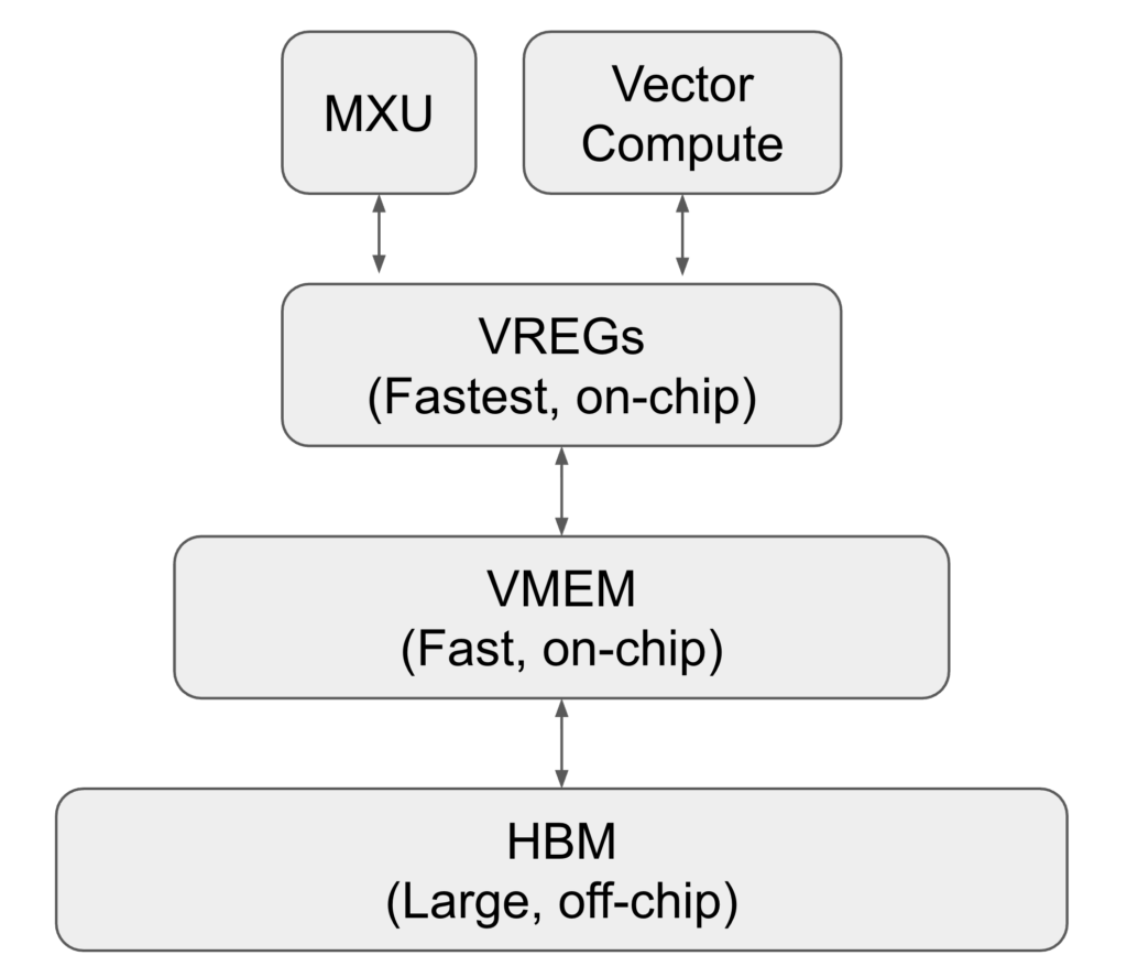
As a result, TPUs feature a memory hierarchy that kernel authors must deeply understand, so that the kernels they write can orchestrate when and how data is loaded from the off-chip HBM to the fast on-chip VMEM. A performant Pallas kernel would overlap these HBM<>VMEM memory transfers with floating point computation happening in the matrix (MXU) and vector compute units.
Despite the architectural differences, current-generation TPUs and GPUs are highly comparable in raw performance. TPU7x and NVIDIA B200 have very similar BF16 compute TFLOPS and HBM bandwidth — the two most important hardware metrics for modern ML workloads.
Helion’s Pallas Codegen
To extract maximum performance out of a TPU, Helion’s Pallas codegen aims to maximize software pipelining, ensuring that memory transfers and computation overlap as much as possible. This section illustrates Helion’s three-fold strategy for generating pipelined kernels:
- Outer loop: pallas-provided pipelined device invocation (
pallas_call/emit_pipeline) - Inner loop: autotuned between:
- pallas-provided pipelined device-side loop (
emit_pipeline) - Pre-fetching all values into VMEM, if possible (
unroll)
- pallas-provided pipelined device-side loop (
- Auto-tuned pipeline buffer sizes
Example: add
As a simple example, consider the following helion kernel for adding two tensors.
@helion.kernel
def add(x: torch.Tensor, y: torch.Tensor) -> torch.Tensor:
    out = torch.empty_like(x)
    for tile in hl.tile(out.size()):
        out[tile] = x[tile] + y[tile]
    return out
The Helion compiler translates this into two functions: a host-side launcher that tiles the input and invokes the device function in a pipelined fashion, and a device function that operates on VMEM-resident tiles:
def _helion_add(x, y, out):
    out[:] = x[:] + y[:]

def add(x: torch.Tensor, y: torch.Tensor):
    _BLOCK_SIZE_0 = <autotuner-selected value>
    out = torch.empty(...)
    out = launcher( # wraps around pallas_call
        _helion_add,
        ((x.shape[0] + _BLOCK_SIZE_0 - 1) // _BLOCK_SIZE_0,), # grid size
        x, y, out,
        _block_spec_info=[_BLOCK_SIZE_0, ...], ...
    )
    return out
Within the generated code:
- The
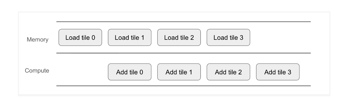
hl.tileloop in the Helion source becomes a grid on the host side. The launcher (wrappingpallas_call) invokes_helion_addonce per tile, with each invocation automatically pipelined — while one tile is being computed, the next tile’s data is being loaded from HBM into VMEM. - The device function
_helion_addis simple: it receives VMEM references (not HBM pointers), so the kernel body is a simple addition. _BLOCK_SIZE_0(the tile/buffer size) is selected by the autotuner, which explores different sizes to find the best overlap between memory transfers and compute for the target hardware.
This results in a pipelined execution as illustrated below.
Example: Flash Attention
Attention is one of the key operations in modern language models. Production implementations follow the “Flash Attention” pattern – a memory-efficient technique that computes attention in tiles to avoid materializing the full S×S attention matrix. The structure of a flash attention kernel in Helion is illustrated below:
B, H, S, D = 8, 32, 8192, 256 # batch, head, sequence length, head dimension
@helion.kernel
def attention(q: torch.Tensor, k: torch.Tensor, v: torch.Tensor) -> torch.Tensor:
    out = torch.empty(...)
    for tile_b, tile_q in hl.tile(B * H, S):
        this_q = q[tile_b, tile_q, :]
        acc = ...
        for tile_kv in hl.tile(S):
            this_k = k[tile_b, tile_kv, :]
            this_v = v[tile_b, tile_kv, :]
            <qk matmul, online softmax, v matmul, update acc>
        out[tile_b, tile_q] = acc
    return out
Compared to the “add” example discussed previously, the flash attention kernel contains an additional inner loop which performs tiled accesses across the entire K and V sequences. How we pipeline the memory and compute within the inner loop is key to the performance of this kernel.
In Helion, the compiler autotunes over two different strategies for translating this kernel to Pallas. This is keyed on the pallas_loop_type autotuner config.
With the default pallas_loop_type == emit_pipeline option, Helion relies on Pallas’ device-side emit_pipeline API to pipeline an inner loop body function, similarly to how the host-side logic uses pallas_call to pipeline the device function invocation:
def _helion_attention(q_VMEM, k_HBM, v_HBM, out_VMEM):
    acc = ...
    this_q = q_VMEM[:, :, :]
    def _inner_pipeline_body(k_VMEM, v_VMEM):
        this_k = k_VMEM[:, :, :]
        this_v = v_VMEM[:, :, :]
        <matmul, online softmax, matmul, update acc>
    pallas.tpu.emit_pipeline(_inner_pipeline_body, k_HBM, v_HBM, _block_spec_info=[BLOCK_SIZE_KV ,...], ... )
    out_VMEM = acc

def attention(q: torch.Tensor, k: torch.Tensor, v:torch.Tensor):
    out = torch.empty(...)
    out = launcher( # wraps around pallas_call
        _helion_attention,
        q, k, v, out,
        _block_spec_info=[BLOCK_SIZE_Q ,...], ...
    )
    return out
This generated kernel follows a nested pipeline structure:
- (Outer pipeline) The host uses
pallas_callto invoke_helion_attention. The HBM reference of q is tiled, and each invocation of_helion_attentionreceives a VMEM tile of q. For k and v,_helion_attentionreceives HBM references directly. - (Inner Pipeline) Within
_helion_attention, the device usesemit_pipelineto invoke_inner_pipeline_body, which receives VMEM tiles of k and v.
This results in a pipelined execution as illustrated in this image:
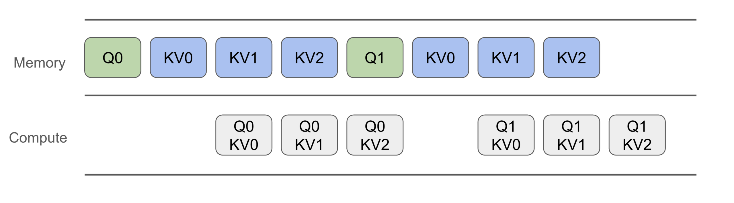
One obvious point of inefficiency in this pipeline is that there are bubbles in the compute units – for every new Q tile, while we fetch the 0th KV tile, there is no work available for the compute units. This comes down to the fact that we are re-loading the KV tiles from HBM to VMEM for every new Q tile.
Helion offers an alternative pallas_loop_type == unroll config which avoids this bubbling. With unroll, we translate the inner for loop into a simple Python for loop:
def _helion_attention(q_VMEM, k_VMEM_FULL, v_VMEM_FULL, out_VMEM):
    acc = ...
    this_q = q_VMEM[:, :, :]
    for offset in range(0, k_VMEM_FULL.size(1) , BLOCK_SIZE_KV):
        this_k = k_VMEM_FULL[:, pallas.dslice(offset, BLOCK_SIZE_KV), :]
        this_v = v_VMEM_FULL[:, pallas.dslice(offset, BLOCK_SIZE_KV), :]
        <matmul, online softmax, matmul, update acc>
    out_VMEM = acc

def attention(q: torch.Tensor, k: torch.Tensor, v:torch.Tensor):
    out = torch.empty(...)
    out = launcher( # wraps around pallas_call
        _helion_attention,
        q, k, v, out,
        _block_spec_info=[BLOCK_SIZE_Q, None, None], ...
    )
    return out
(The name “unroll” reflects the fact that Pallas device functions are traced by JAX’s JIT — the Python for loop is effectively unrolled at trace time into a flat sequence of operations.)
In this version of the generated kernel:
- K and V are pre-fetched in full: The host passes
Noneas the block spec for K and V, instructingpallas_callto load them entirely into VMEM. The full VMEM references persist across all device function invocations. - The inner loop slices locally: Each iteration uses
pallas.dsliceto select the relevant KV tile from the already-resident VMEM buffer. No HBM traffic occurs during the inner loop.
This results in a different pipelining scheme as illustrated below:
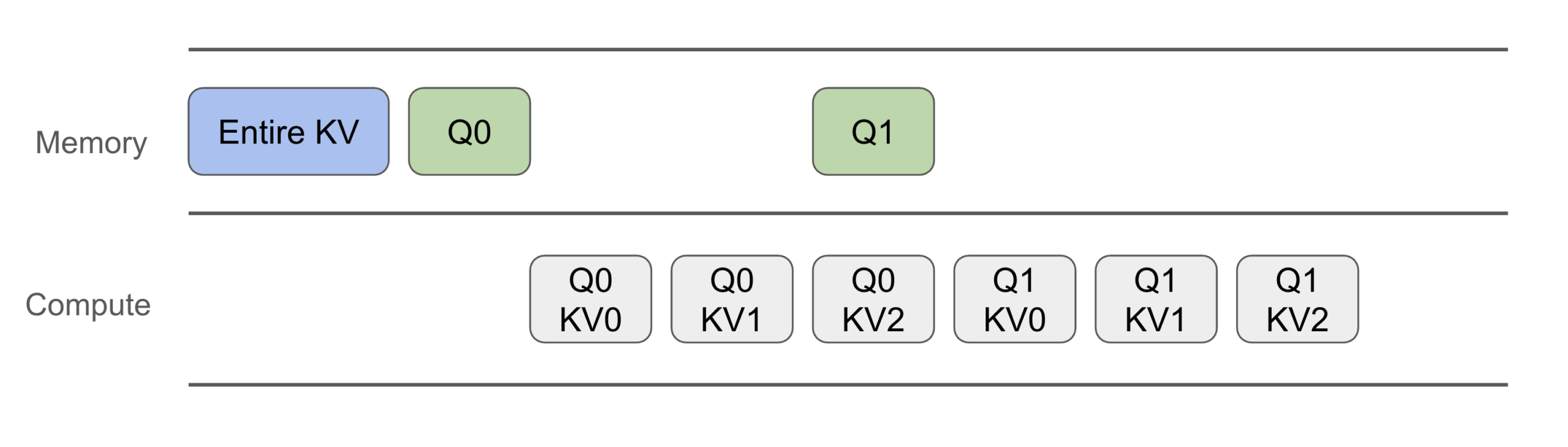
In this workflow, there are no longer bubbles in the compute pipeline. The trade-off is that this requires more VMEM usage, as the entire K and V sequences need to be present. This means that although more performant, this translation isn’t always possible. The VMEM usage is linear with respect to the input sequence lengths (as opposed to tile size), which is prohibitive with longer sequences. The performance difference between these strategies is significant — the table below shows results on workloads with B=8, H=32, D=256:
| S = 8k | S = 32k | |
|---|---|---|
| emit_pipeline TFLOPs | 653 | 695 |
| unroll TFLOPs | 892 | OOM |
The benefit of Helion lies in its ability to autotune and select the best autotuner config. So that with smaller sequences, it makes use of the VMEM available and generates pipelined code with no compute bubbles. For longer sequences, it falls back to emit_pipeline which scales to arbitrary context lengths. The following graph plots the performance of this attention kernel compared to various other Pallas attention implementations, on varying sequence lengths:
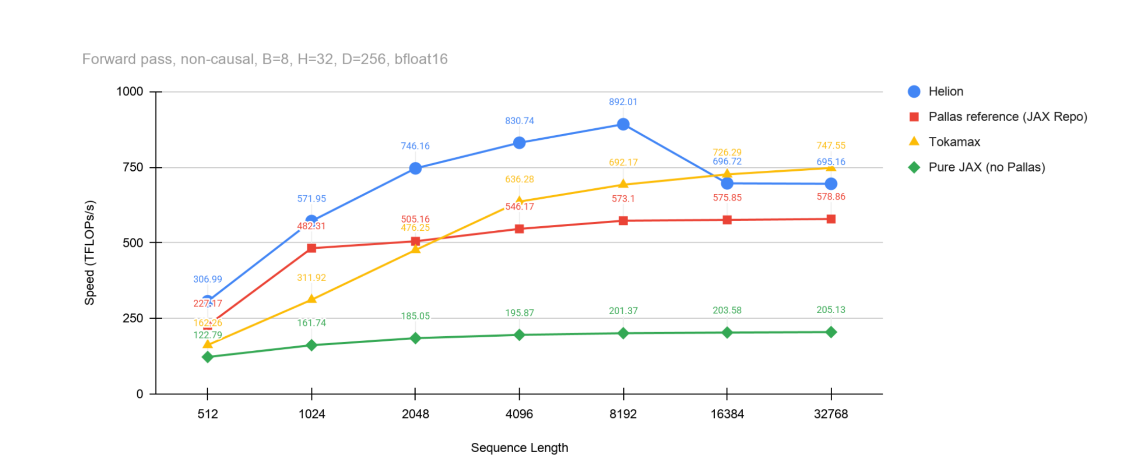
The autotuner’s ability codegen different loop and pipelining strategies depending on the input length is what gives Helion its edge even when compared to highly optimized implementations such as Tokamax.
Broader Kernel Benchmarks
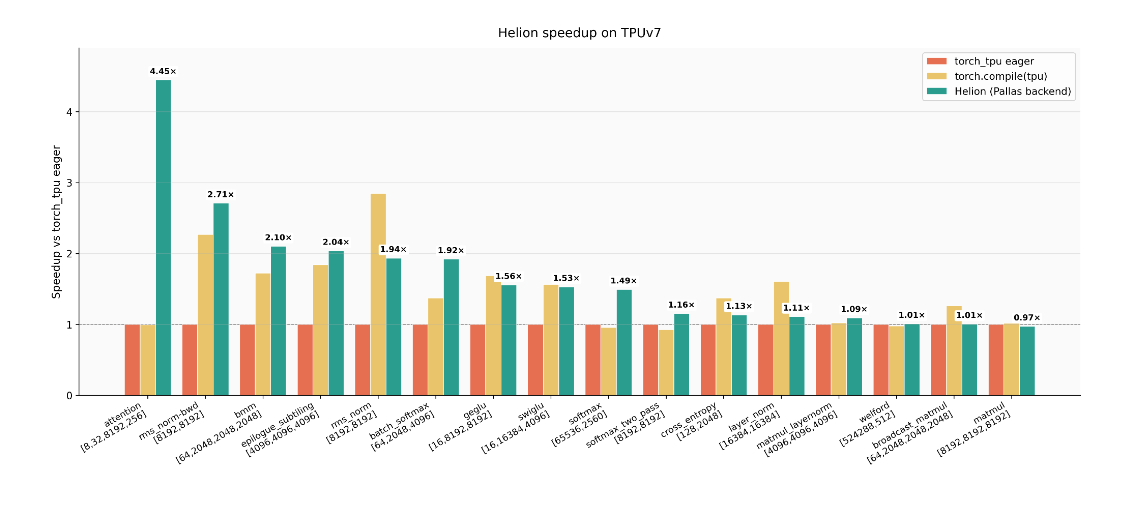
We benchmark Helion across a variety of kernels, tracked on our dashboard. The table below compares Helion against TorchTPU eager and torch.compile (using XLA) across a range of different kernels. Helion shows a geometric average speed-up of 1.55x compared to eager, and 1.12x compared to compiled.
| kernel | shape | torch_tpu eager (ms) | torch.compile(tpu) (ms) | Helion (ms) | Helion vs torch_tpu eager | Helion vs torch.compile |
|---|---|---|---|---|---|---|
| attention | [8,32,8192,256] | 87.77 | 88.28 | 19.72 | 4.45× | 4.48× |
| softmax | [65536,2560] | 0.712 | 0.743 | 0.477 | 1.49× | 1.56× |
| batch_softmax | [64,2048,4096] | 1.888 | 1.373 | 0.982 | 1.92× | 1.40× |
| softmax_two_pass | [8192,8192] | 0.386 | 0.417 | 0.334 | 1.16× | 1.25× |
| bmm | [64,2048,2048,2048] | 3.211 | 1.860 | 1.527 | 2.10× | 1.22× |
| rms_norm-bwd | [8192,8192] | 1.792 | 0.789 | 0.661 | 2.71x | 1.19x |
| epilogue_subtiling | [4096,4096,4096] | 0.850 | 0.462 | 0.417 | 2.04x | 1.11x |
| matmul_layernorm | [4096,4096,4096] | 0.535 | 0.523 | 0.489 | 1.10× | 1.07× |
| welford | [524288,512] | 1.330 | 1.357 | 1.316 | 1.01x | 1.03x |
| swiglu | [16,16384,4096] | 3.510 | 2.244 | 2.295 | 1.53× | 0.98× |
| matmul | [8192,8192,8192] | 1.552 | 1.527 | 1.597 | 0.97× | 0.96× |
| geglu | [16,8192,8192] | 3.779 | 2.240 | 2.424 | 1.56× | 0.92× |
| cross_entropy | [128,2048] | 0.363 | 0.264 | 0.320 | 1.13× | 0.82× |
| broadcast_matmul | [64,2048,2048,2048] | 1.817 | 1.440 | 1.806 | 1.01× | 0.80× |
| layer_norm | [16384,16384] | 1.253 | 0.779 | 1.126 | 1.11× | 0.69× |
| rms_norm | [8192,8192] | 1.194 | 0.419 | 0.617 | 1.94× | 0.68× |
Helion shows the largest gains on kernels that employ fusion or optimization patterns that are difficult for XLA to discover automatically — flash attention is a prominent example. For the more standard operations like matmul and layer_norm, XLA’s compiler already produces high-quality code, and Helion performs comparably.
What’s Next
Helion on TPU is under active development. Here’s a non-exhaustive list of things we are working on:
- Expand kernel coverage: Get more Helion examples working on TPU
- Further performance improvements
- Better support for jagged and sparse operations
- Support for distributed TPU computing
Getting Started
Helion is open source and available on GitHub. Its TPU backend has a dependency on TorchTPU, which is expected to be released publicly later this year. When it does, we encourage you to try-out Helion on TPU and share your feedback. Resources:
Acknowledgements
This project was made possible through the invaluable collaboration and technical insights of our peers. A special thank you to Joe Pamer, Robert Hundt, Claudio Basile and Adam Paszke at Google, as well as Jana van Greunen, Gregory Chanan, Peng Wu, and Zongwei Zhou at Meta, for their feedback and support in bringing this to fruition.
0 Comments
Log in to join the conversation.No comments yet. Be the first to share your thoughts.