Extended Connectivity Fingerprint in APL

Citing the Rogers and Hahn paper1 is a rite of passage for everyone in cheminformatics. This post tries to faithfully implement Extended Connectivity Fingerprint (ECFP). I will not be making any effort explaining exactly how and why ECFP is as popular as it is. There are probably at least a dozen papers every year where ECFP baseline seems suspiciously good compared to <insert your favorite million-parameter embedding model>.

The goal of this post is twofold: 1. To crudely explain how ECFP works, 2. To implement it in APL (and NumPy to verify if it’s correct).

I’m sure most of you either love, hate or have no clue about APL. So, I’ll leave the learning part of this language as an exercise to the reader, hehe. I have read and learnt what I’ll be using here from Mastering Dyalog APL (which I think is very well written and easy to understand).

Before I ramble on any more, I’d like to refer the reader to these excellent resources that have already done a great job at explaining ECFP:

1. https://depth-first.com/articles/2019/01/11/extended-connectivity-fingerprints/

2. https://cdpkit.org/cdpl_python_cookbook/descr/fingerprints/ecfp.html

3. https://www.blopig.com/blog/tag/extended-connectivity-fingerprints/

4. https://medium.com/@musicalchemist/from-theory-to-code-a-deep-dive-into-molecular-extended-connectivity-fingerprints-ecfps-with-da1ed436925e

5. https://chemicbook.com/2021/03/25/a-beginners-guide-for-understanding-extended-connectivity-fingerprints.html

6. https://docs.chemaxon.com/latest/fingerprints_extended-connectivity-fingerprint-ecfp.html

ECFPs are a type of Topological Fingerprints2. The paper starts with

[…] ECFPs are derived using a variant of the Morgan algorithm […]

So, what is this Morgan algorithm3 ? In plain english, it is a method developed with the intent of developing a computer-based registration system for the Chemical Abstracts Service (CAS) to uniquely identify chemical structures (in the 1960s !!!). The algorithm tries to assign a single, unique alphanumeric description to every two-dimensional chemical structure.

So, back in the mid 60s (I’m saying this as if I was there, anyways), in between the Beatlemania, Civil Rights Movement, Assassinations, Cold War, and most certainly way before SMILES, the most common format for storing chemical structures was the connection table. A connection table is an ordered list that serves as an unambiguous machine description of a chemical structure’s two-dimensional projection. It defines the structure by describing the atomic symbol (or “value”) of each non-hydrogen node alongside its exact bonding attachments to the other nodes in the graph.

To capture these structural relationships, the connection table is organized into five specific lists: the FROM ATTACHMENT (which records the lowest-numbered connected atom), the RING CLOSURE (which accounts for bonds forming cycles), the NODE VALUE (which notes the atomic symbols), the LINE VALUE list (which codes the bond types), and the MODIFICATIONS list (which describes special attributes like ionic charges, isotopic mass, or unusual valence).

The keen readers might already have figured out why this representation could be problematic for search but in case it’s not clear, let’s consider an arbitrary example of this abstract molecule:

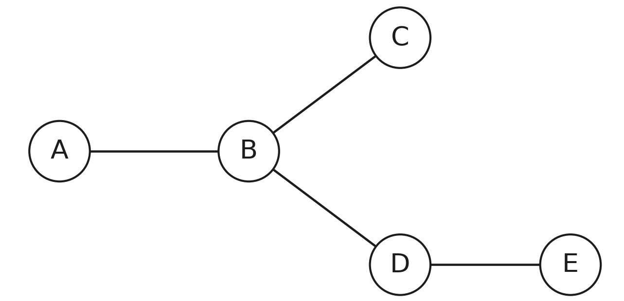
Where do you suppose one should start the table? A, B, C, D or E? And what should be the order of these in the table? Consider what happens if we naïvely try two different numberings. Here they are with their FROM lists side by side:

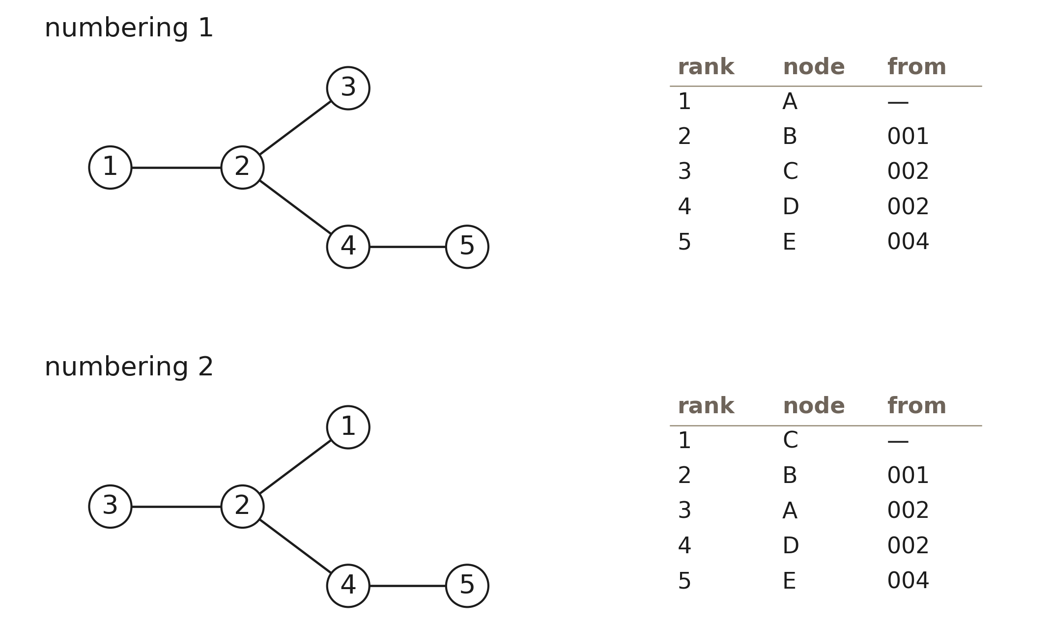
Now, let me be clear, I only showed two graph orderings here, but technically the space of ordering looks more like this5 :

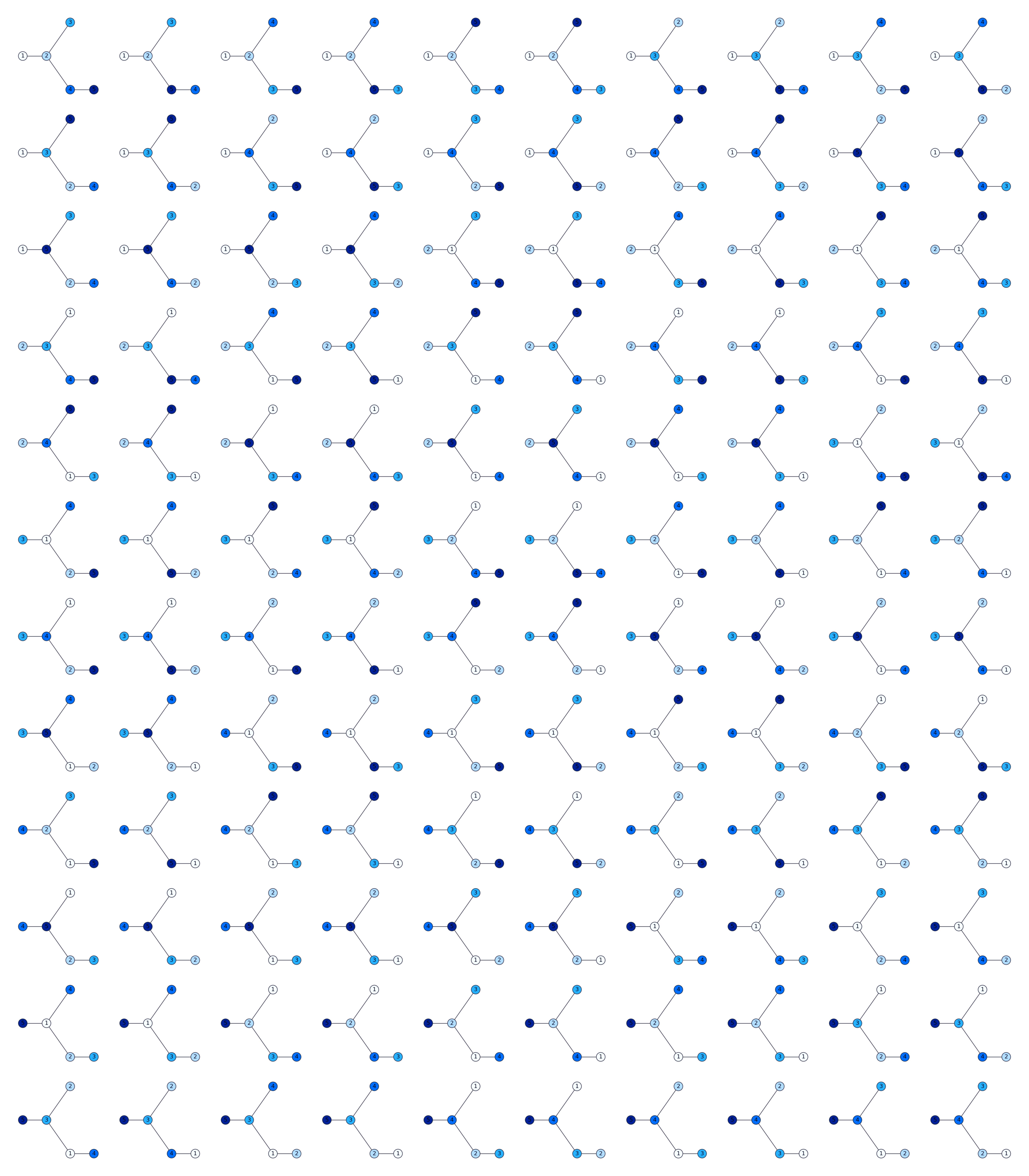
In case you are still not convinced, let’s try to look at the number of unique enumerations of graph based on number of nodes. This function is the factorial (!)

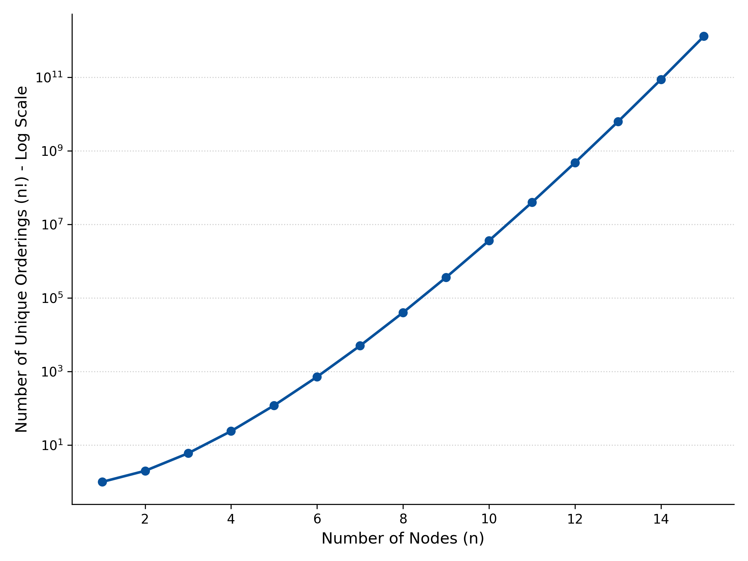
So this brute-force enumerate-search idea is silly to say the least. Now, if there was a way such that you could take in an arbitrary connection table / graph and arrange or order it always in the same way for a given molecule, that would solve our problem. This is exactly what Morgan did.

I will now stop using this table analogy and instead we should think of this as a graph theory problem (just because it sounds fancy and cool). This problem can be thought of as either the graph canonization problem (i.e. given a graph, output a canonical labelling of its vertices, one that depends only on the graph's structure) or the graph isomorphism problem (i.e. given two graphs, decide whether they are the same upon relabelling). Canonization is the “stronger” of the two i.e. if you can canonize, you can decide isomorphism for free by canonizing both graphs and comparing them. Either way, the idea that for a given graph there exists a function that will canonically order its nodes is an opportunity to solve our problem. But before we get too excited about this, let's actually see how Morgan proposed to do it.

Morgan algorithm simply is following these steps iteratively:

1. Give each heavy atom an initial connectivity value and call it EC value, for extended connectivity, yes these are the first two words in ECFP indeed. This is important: We create a variable k which is the number of unique EC values in the molecule. E.g. If the list of EC values is [1,2,3,4,4] then k is 4. For those who speak python, this is simply :

2. For every atom, compute its updated EC value as the sum of EC values of its neighbors. Call this number of distinct updated values k’.

3. If k’ > k, replace the old EC values with the updated ones, set k as k’, and repeat step 2.

4. If k’ ≤ k, break the loop, i.e. stop. The invariants Morgan actually uses are the values from the previous iteration i.e. the last one at which k strictly increased.

When the process terminates, the values from the terminating iteration are thrown away (subtle foreshadowing, hehe). What you keep is the last set of values that increased k. Morgan called this “the last set of values assigned to the nodes”. And that’s what all the downstream tie-breaking (partial ordering, canonical numbering, the connection table itself) is built on top of.

Confused ? Well, see this iterative process on caffeine:

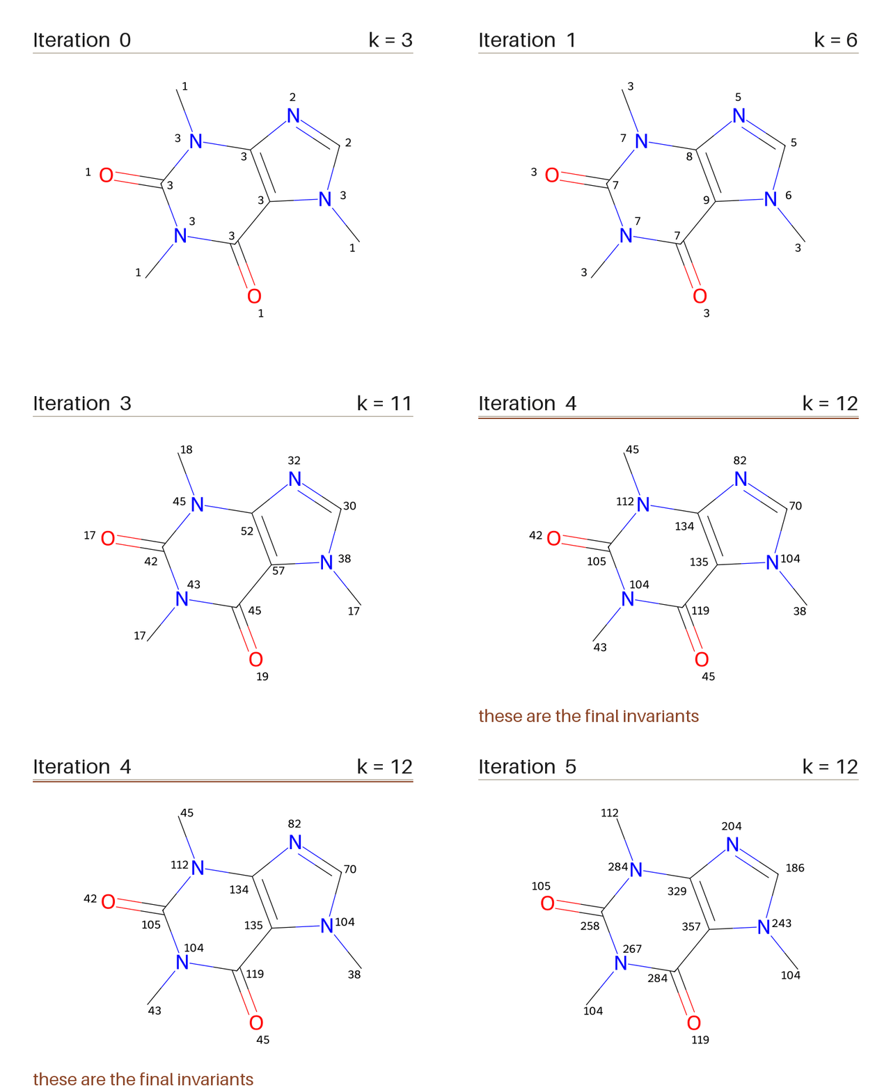
Iteration 0 is just the heavy-atom’s degree. Iteration 1 passes / spreads structural context outward: an atom’s value now depends on how connected its neighbors are. By iteration 3, atoms that “look different from a distance” i.e. near an oxygen, near two nitrogens, inside the fused ring, etc. carry very different values. The process quits when refining further stops providing new equivalence classes, and it just hands back the previous iteration’s values.

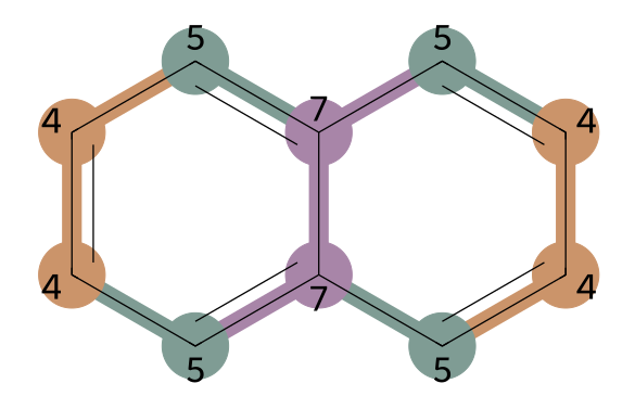
The pleasant side of the story is that whenever the graph has a real structural difference between two atoms, Morgan usually surfaces it. Naphthalene, for instance, partitions cleanly into three equivalence classes: bridgeheads, α-carbons, β-carbons and Morgan finds all three after one iteration:

We can do this on our simple abstract molecule just to make it clearer.

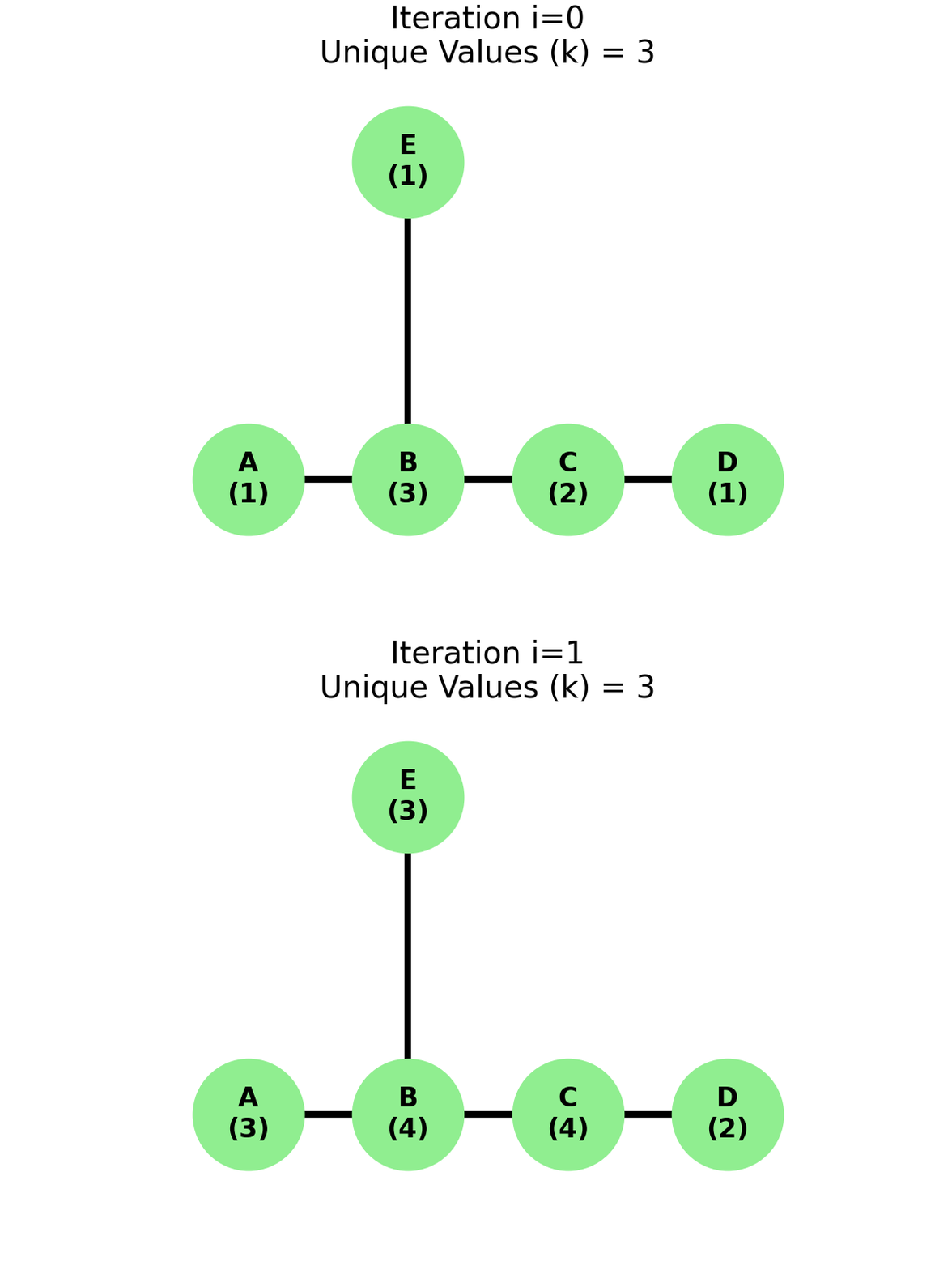
We can let the iterations go on but it’s evident that in this case, the number of unique values doesn’t change. Before you read any further, take a wild guess if you think k not changing with increasing iterations is a general trend always ?

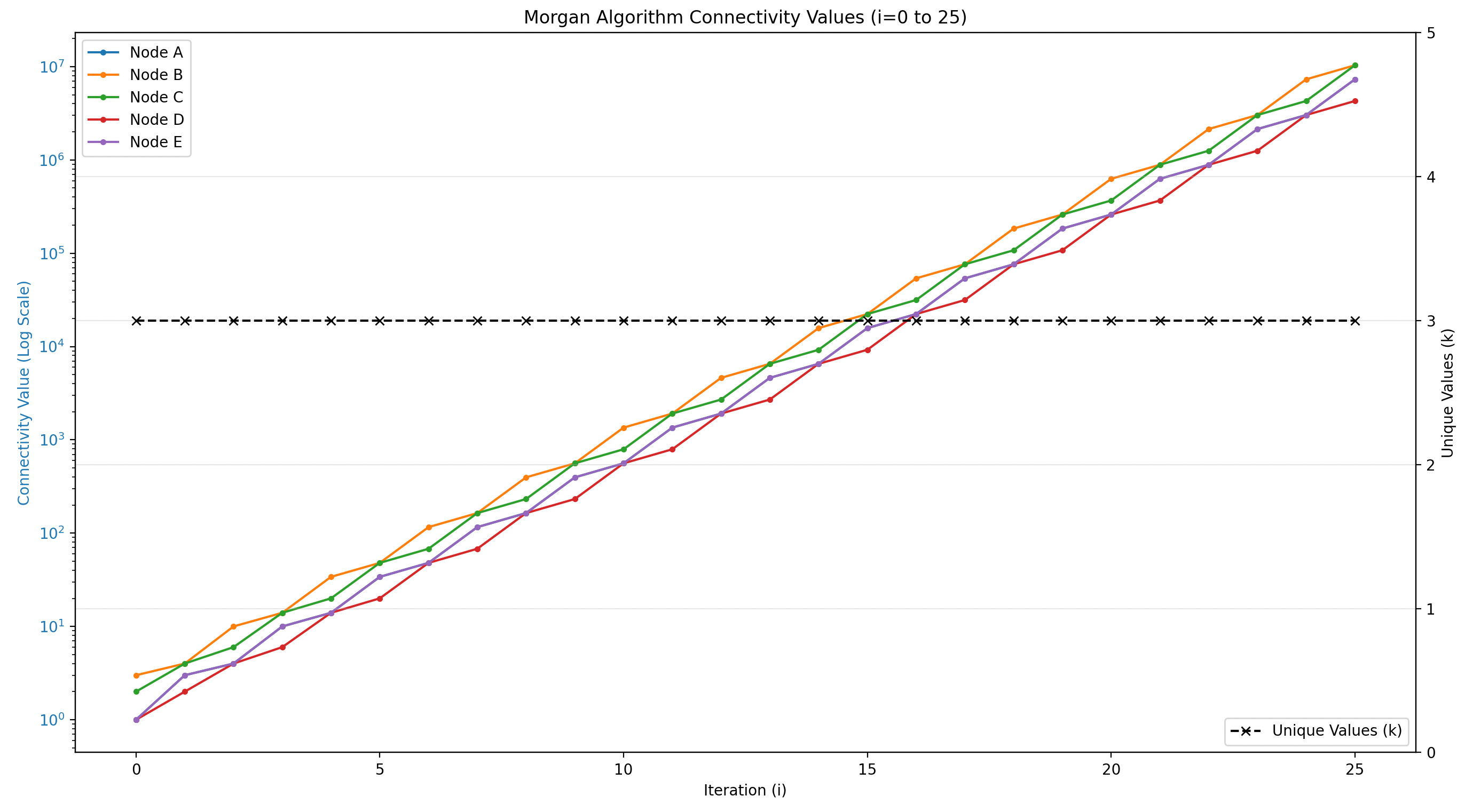
Well if you guessed it’s false, you are absolutely right ! In fact now I will show you a very simple counter example to prove that structurally different nodes can accidentally sum to the exact same number making the stopping condition insufficient.

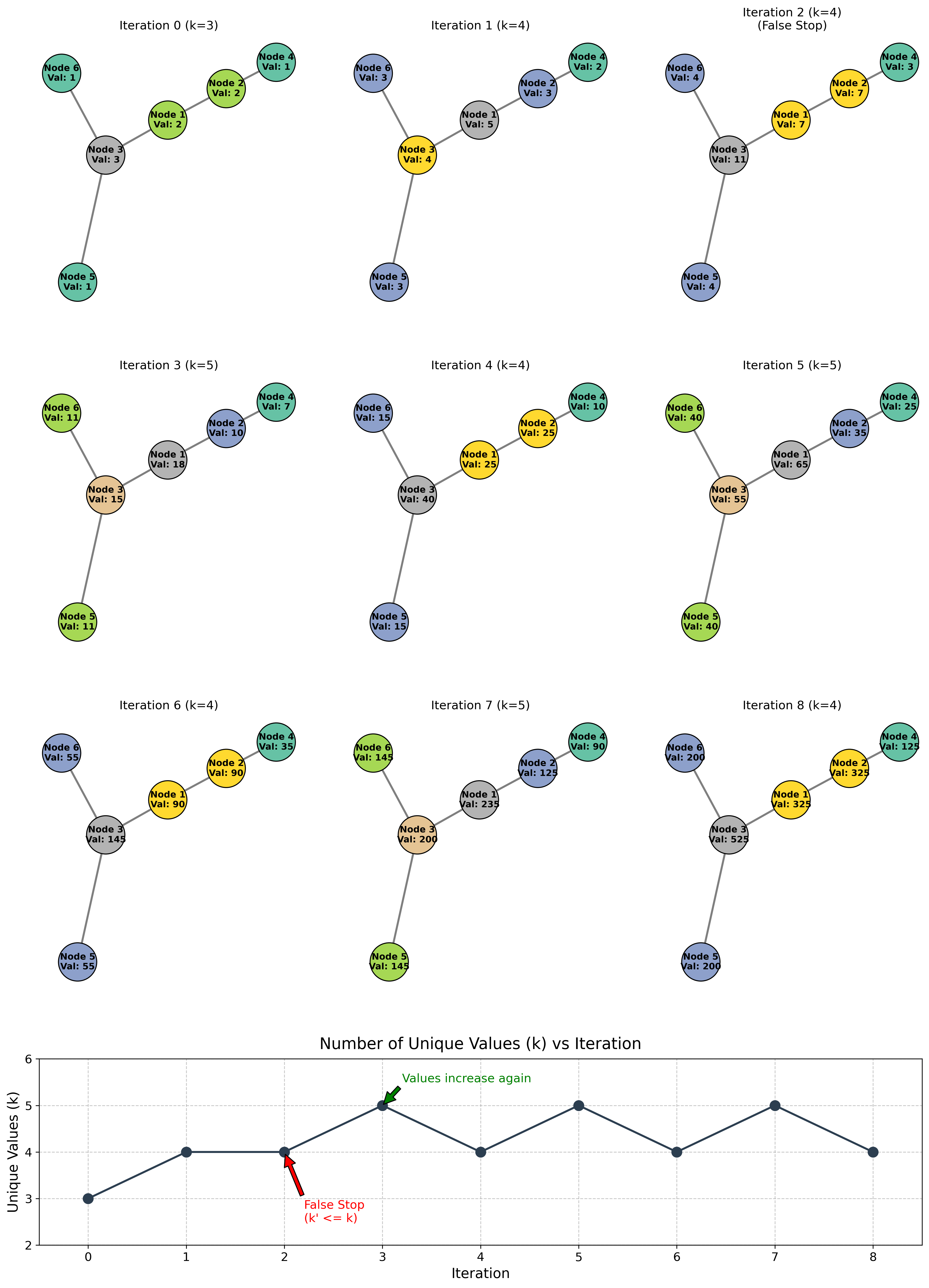
This seems to hint at a more general limitation. Morgan’s update rule reduces the multiset of neighbour values (fancy way of saying all known / considered information of that atom) into a single number by simply adding them up. And a sum is a lossy hash of a multiset (fancy way of saying two different pairs of numbers can have the same sum). So there exist pairs of atoms that are structurally distinguishable (their neighbour multisets differ) but that Morgan will assign the same value to anyway.

In the graph theory literature, this whole family of iterated colour-refinement schemes is known as the Weisfeiler–Leman algorithm (1-WL)8. Morgan algorithm with sum is strictly weaker than 1-WL, and 1-WL itself already has blind spots. Here is the classic one: two 2-regular graphs on six vertices that 1-WL simply cannot tell apart:

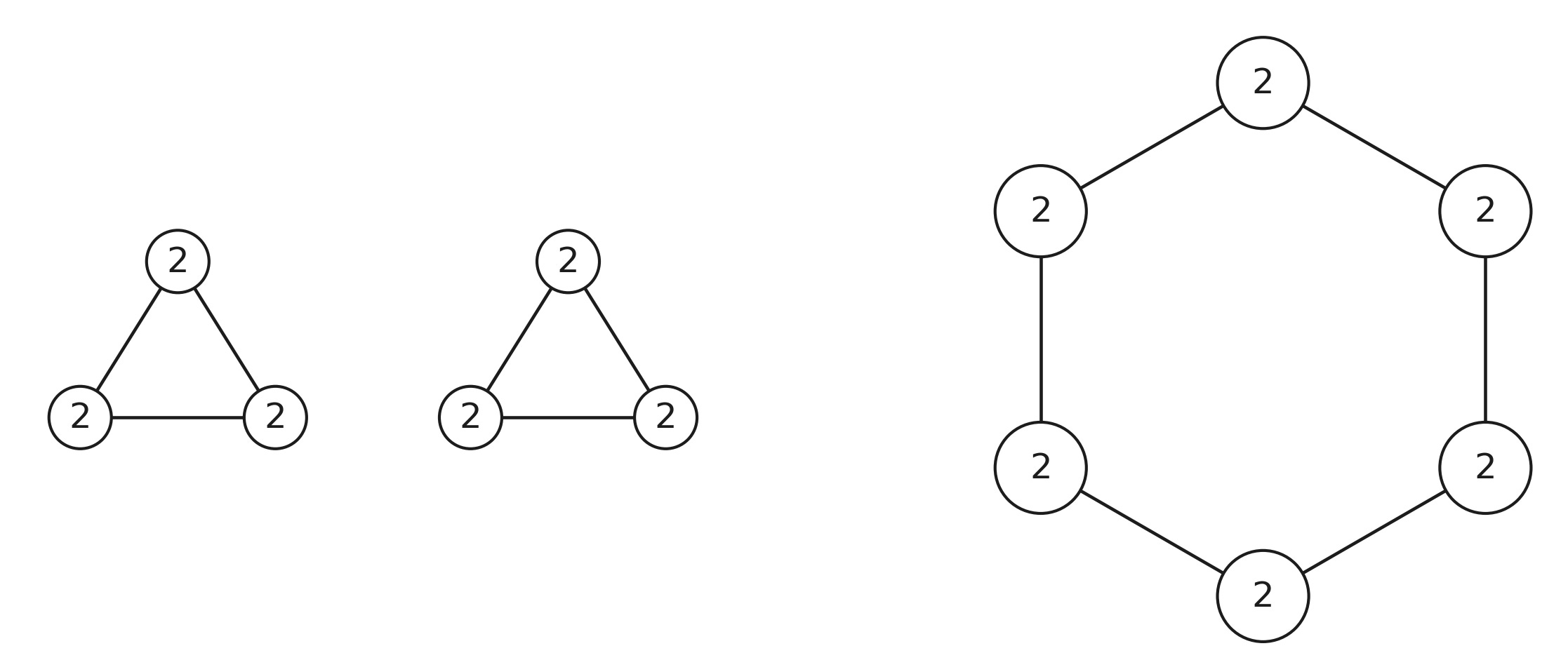
Every node in both graphs has degree 2. Every node’s neighbors in both graphs form the multiset {2,2}. The colour histograms agree at every iteration. But the graphs are obviously different. The one on the left is disconnected. 1-WL cannot see the difference and neither can Morgan !

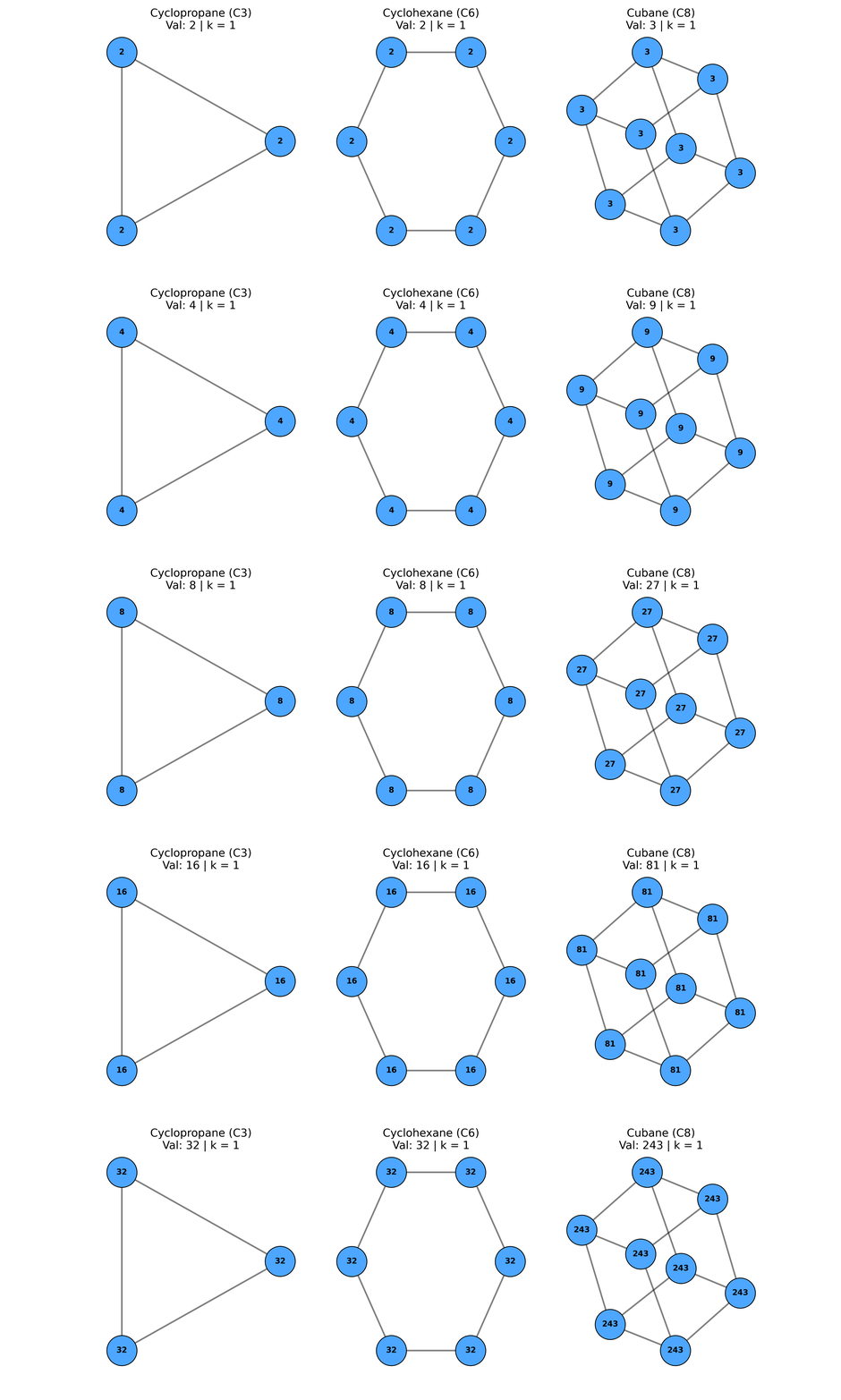
It’s also interesting to see Morgan algorithm applied to highly symmetrical structures. Here for instance, k stays at 1. The six carbons of cyclohexane for instance are symmetric i.e. no canonical procedure should call one of them “position 1” over the others based on structure alone. That symmetry has to be broken arbitrarily (in the original paper, by picking the lowest input index) at the numbering stage, basically randomness at that point.

In all fairness, for the CAS registry that Morgan was building for, none of this actually mattered much. Real drug-like molecules are asymmetric enough that the sum-based invariants almost always split them, and Morgan pins down the residue with a bunch of other tie-breakers (node value = atomic symbol, line value = bond type, look-ahead over terminal atoms, sub-graph splitting on cut bonds).

I hope by now you have some intuition about what Morgan algorithm does and how it works. There are many edge cases and interesting structures that I could show here and discuss at length but let’s try to get back to what this post is actually about, ECFP.

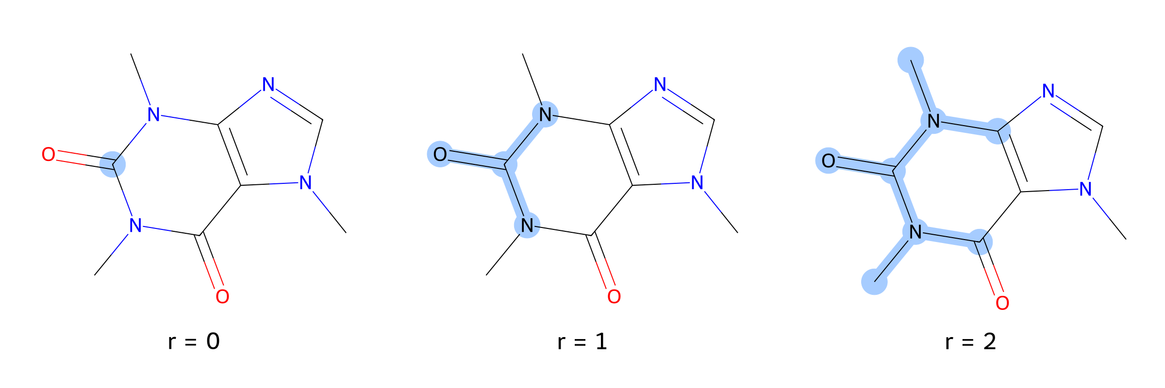
Now, if you re-read that last section with your fingerprint hat on, the interesting bit isn’t the termination criterion. It’s exactly what Morgan algorithm generates along the way. Each iteration produces one integer per atom, and that integer summarizes everything within a radius r around the atom. An integer per atom per radius. If you were feeling greedy, you’d bundle those integers up and use them as a bag of features describing the molecule !

That is essentially what Rogers and Hahn did. From the ECFP paper:

“The ECFP algorithm makes several changes to the standard Morgan algorithm. First, ECFP generation terminates after a predetermined number of iterations rather than after identifier uniqueness is achieved. The initial atom identifiers, and all identifiers after each iteration, are collected into a set; it is this set that defines the extended-connectivity fingerprint. Rather than discarding the intermediate atom identifiers, the ECFP algorithm retains them.”

It’s not a lot, just three modifications, really:

1. Fix the number of iterations up front. For ECFP_N we perform N/2 iterations, where N is the diameter (in bonds) of the largest fragment captured. Each iteration adds one bond of radius, and diameter is twice the radius. Three iterations get you ECFP_6; two iterations get you ECFP_4; and so on.

2. Keep every intermediate. Every atom invariant computed at every iteration lands in a list. This list, deduplicated (set of the list), is the fingerprint.

3. Replace summing with hashing. For each atom, gather the tuple (iteration_level, own_current_invariant, sorted list of (bond_order, neighbour_invariant)) and hash it into a fresh 32-bit int. The neighbour pairs are sorted so the tuple doesn’t depend on how the atoms were laid out.

Modification #3 is the most important one. Summing is a lossy compression of the neighbour multiset. Hashing (with a decent hash function) has essentially zero collision at 32 bits. It also has the pleasant side-effect that the integers are directly comparable across molecules. The substructure inside caffeine and theobromine gets the same identifier in both, because the input tuple to the hash is identical.

The initial identifier at iteration 0 also gets an upgrade. Morgan started from heavy-atom degree which is a very lossy descriptor of an atom. ECFP starts from a hash of the Daylight atomic invariants six properties that are already independent of atom numbering (heavy-atom degree, valence minus attached hydrogens, atomic number, atomic mass, atomic charge, count of attached hydrogens) plus a seventh flag for whether the atom is in a ring. Iteration 0 of ECFP therefore already distinguishes, for instance, carbon-in-aromatic-ring from carbon-in-carbonyl.

There is one more piece to this i.e. duplicate structural removal. Two atoms in the same molecule can end up with different hashed identifiers that actually cover the same set of bonds.

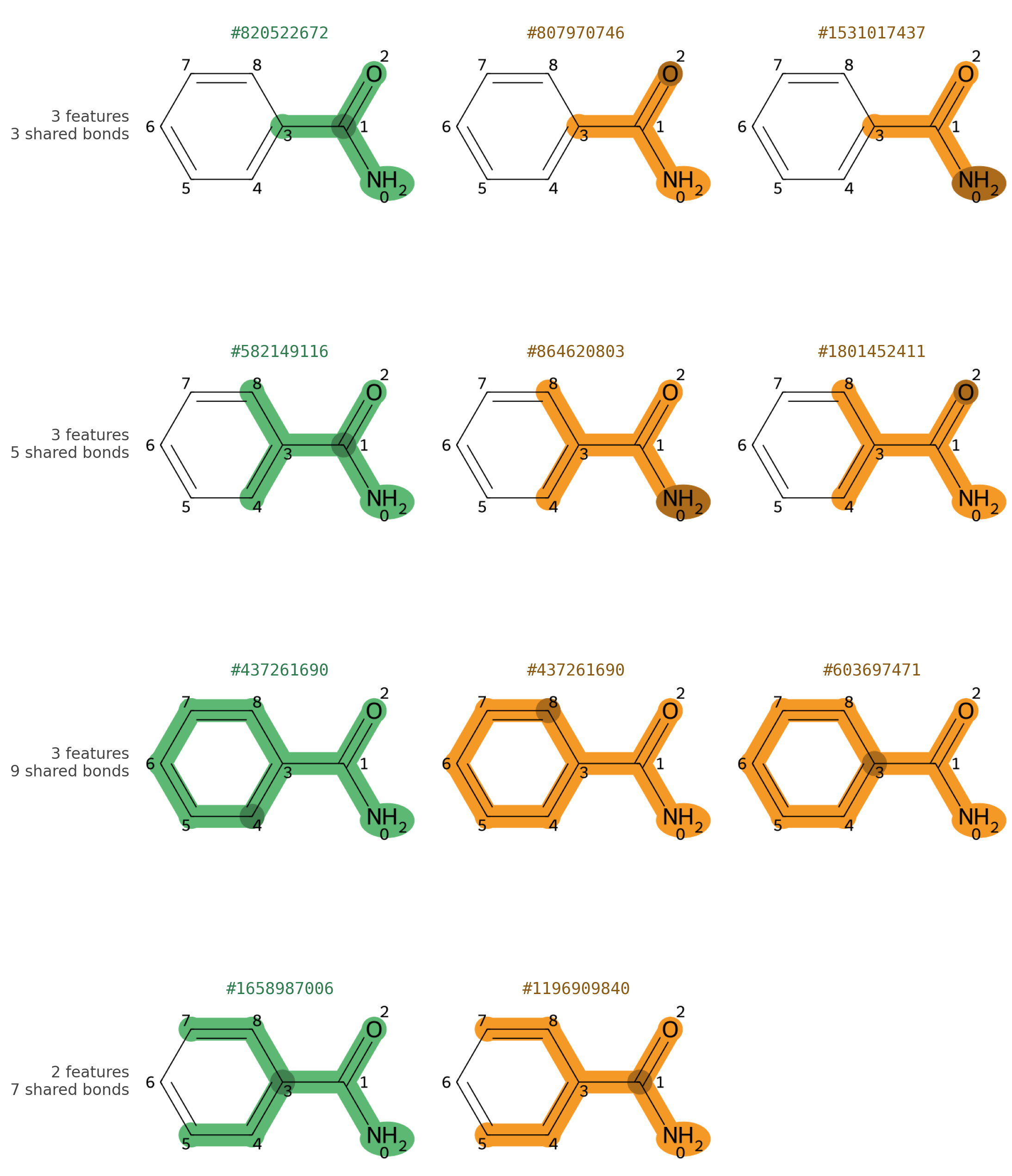
Benzamide is a good place to watch it happen. Grow the neighborhoods out a couple of bonds and you find features centered on different atoms landing on the very same fragment. Same substructure, different identifiers, so at least one is redundant. We keep the feature from the earliest iteration (and, on a tie, the smaller identifier) and drop the rest.

Now I need to introduce you to how I’m planning to verify what I’m doing is actually correct. The easiest way that comes to my mind is to let RDKit do two favors for me. First, hand it a SMILES and get the per-atom invariants and the bond-weighted adjacency matrix (unless you want me to implement OpenSMILES parser, etc. in APL. I will actually get a kick out of doing that, but that’s for some other day, I guess). Second, let it compute its own Morgan fingerprint on the same molecule, so I have something to compare against (along with the NumPy implementation which should return the same outputs as APL).

The two implementations (NumPy and APL) share nothing other than the definition of the hash and the order in which things get hashed, so if they are in agreement it mostly means I’ve done something right, at least that’s my thought process right now.

SMILES → Invariants → Save as a CSV → Algorithm Implementation → Fingerprint

The only things ECFP needs from chemistry side of things are the seven invariants per atom. The six Daylight invariants plus a ring flag and the bond orders.

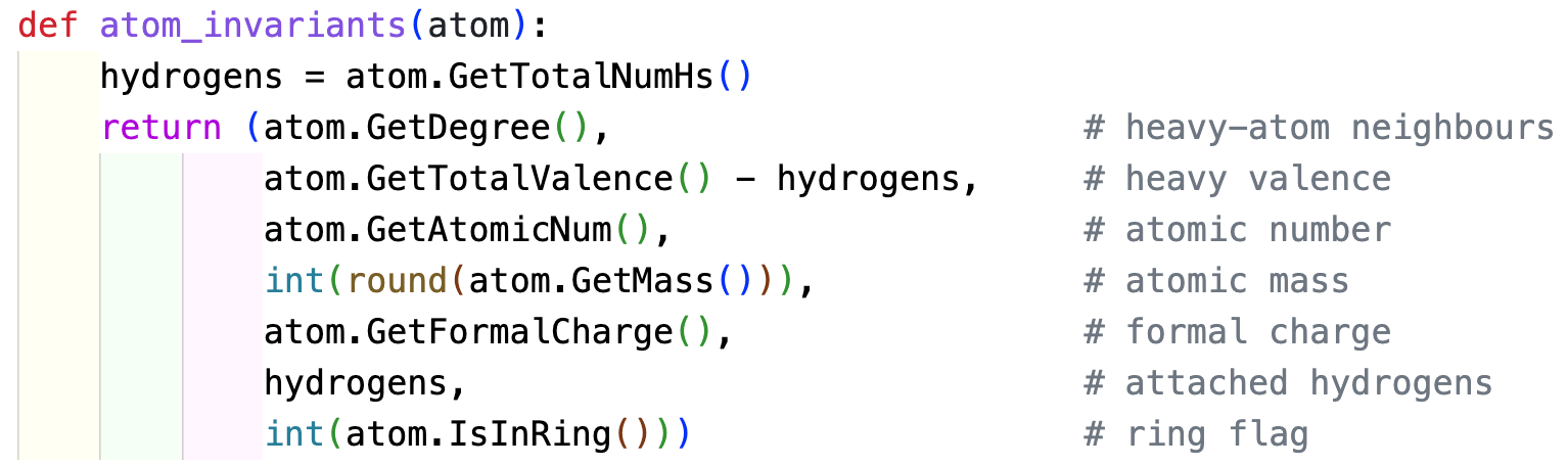
Every one of these is node order-independent i.e. it depends only on the atom, not on where the atom happened to land in the atom list. Iteration 0 of ECFP is just a hash of this tuple.

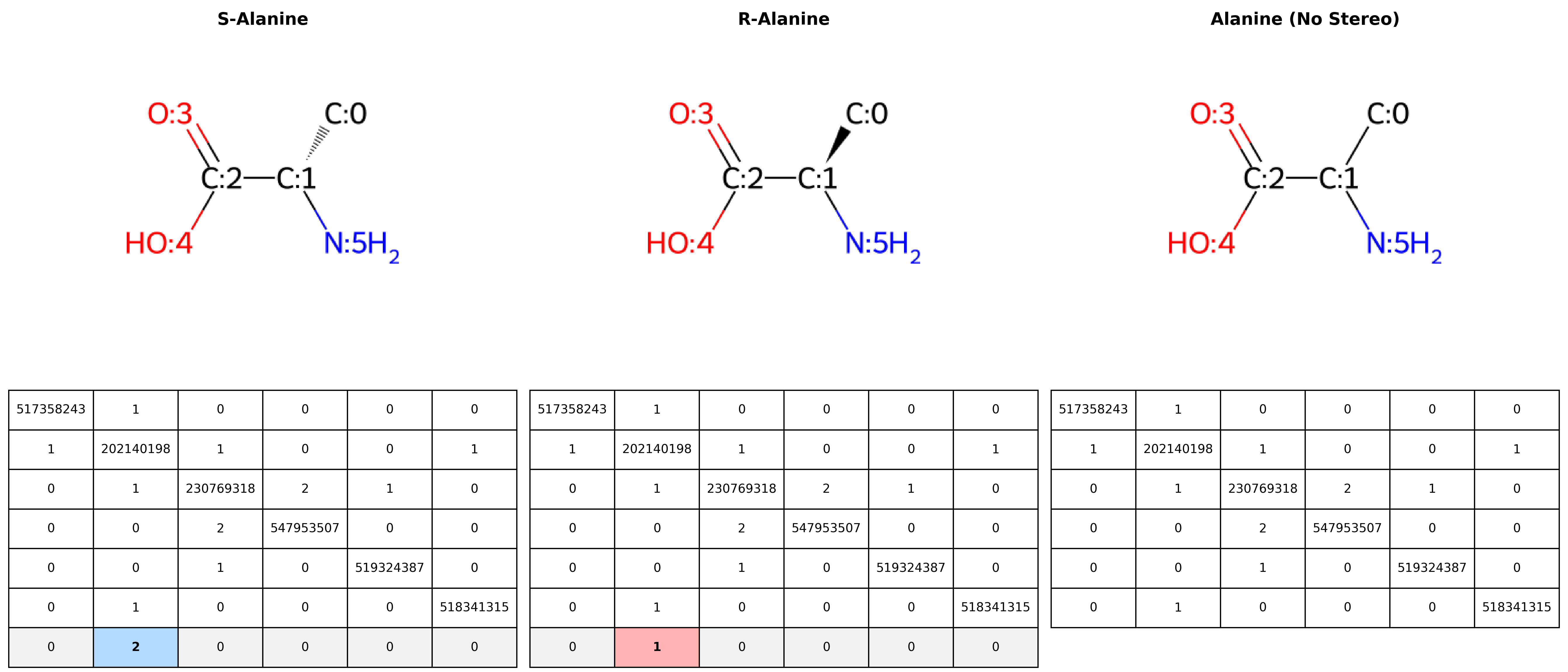
The molecule is stored as an integer matrix. The diagonal holds each atom’s initial identifier (the hash of its invariants) and the off-diagonal holds bond orders (1, 2, 3, 4 for single, double, triple, aromatic).

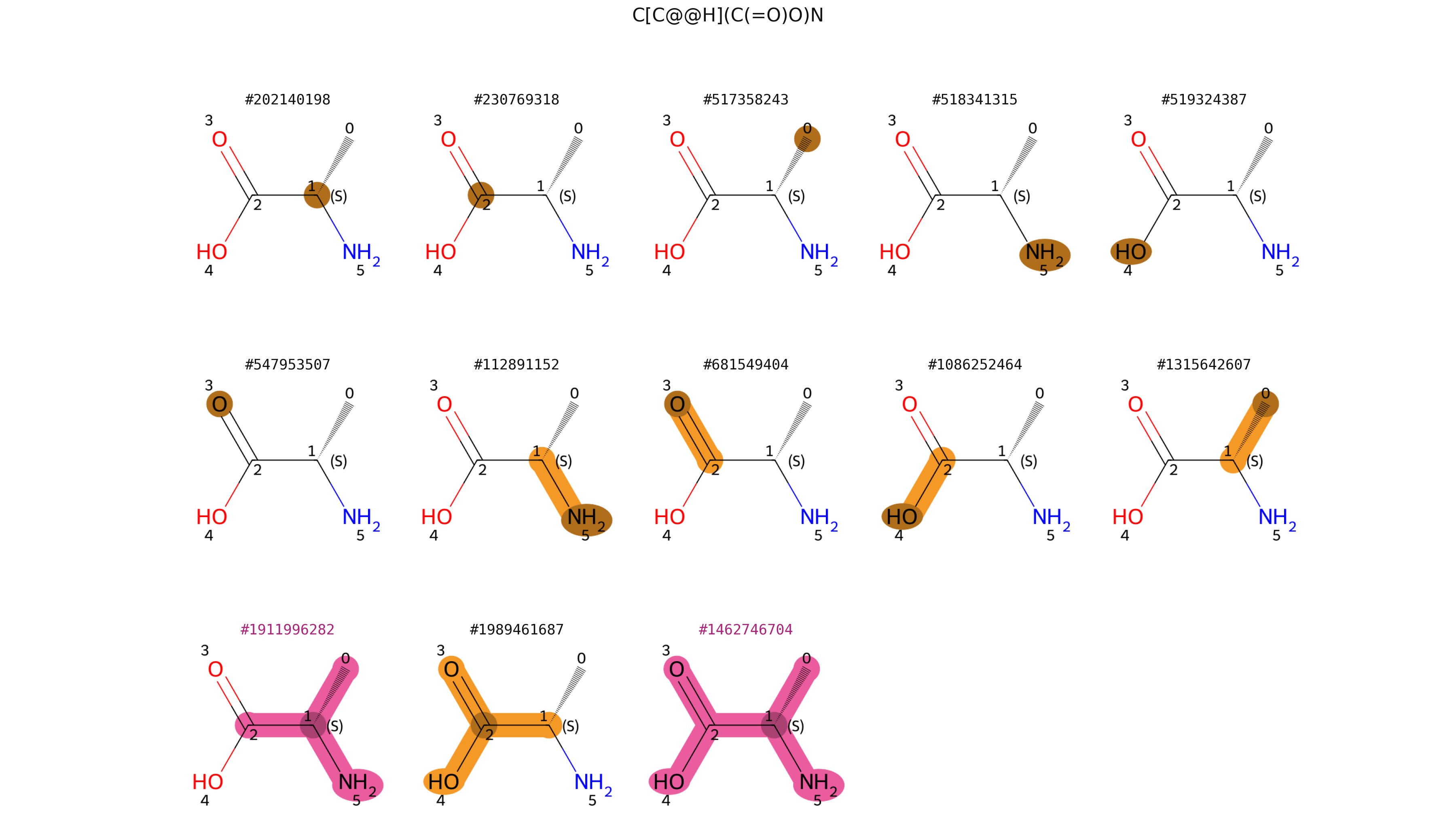
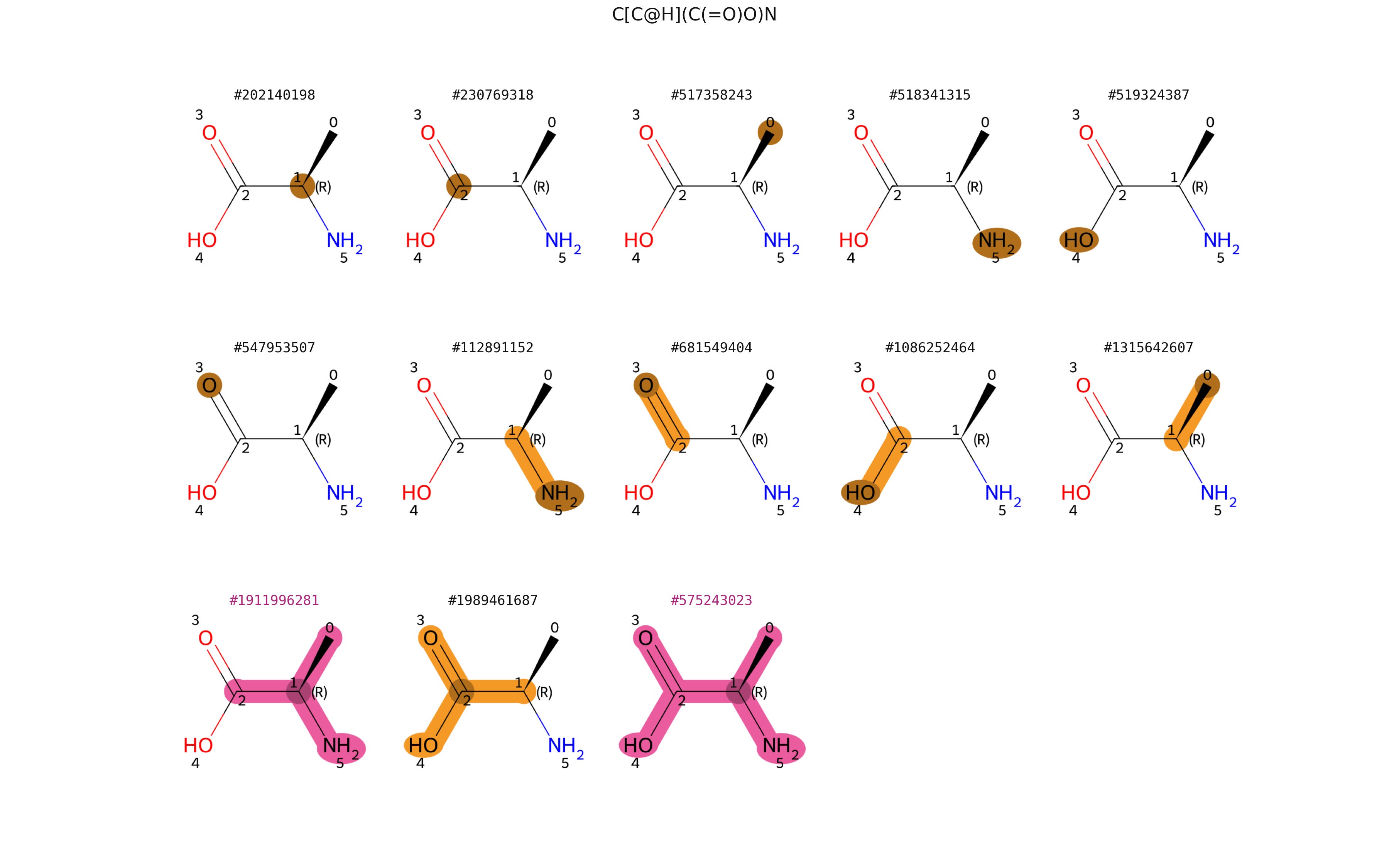
Note: symmetric bond-order adjacency matrix encodes connectivity but not handedness. There is no entry in it that distinguishes R from S. To carry stereochemistry, I’ve added one extra row. That row is a per-atom parity code: 0 for a non-stereocenter, 1 for R, 2 for S.

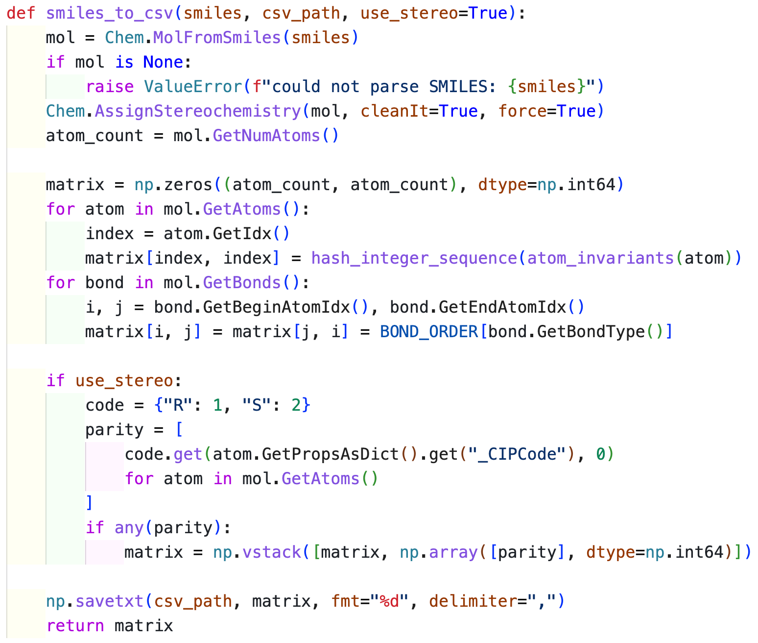
CIP labels are canonical, so the parity row is numbering-independent like the rest of the matrix. A square matrix therefore describes an achiral molecule, and two enantiomers differ only in this final row. I’m sure there are ways to do this in the matrix itself but come on, this is way easier.

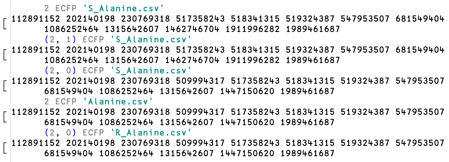
Just to confirm everything is correct, let’s run this thing with S-Alanine (C[C@@H](C(=O)O)N), R-Alanine (C[C@H](C(=O)O)N) and Alanine without any stereochemistry specified (CC(C(=O)O)N).

Before either implementation, I need a hash function, and I need the same hash in Python and APL given the same input. The following is nerd talk that most of you can skip. I learnt that unlike Python, Dyalog APL’s integers turn into floats above 253, so a proper 32-bit hash with a multiply-heavy mixer will overflow that line in one language and not the other. So what can I do ?

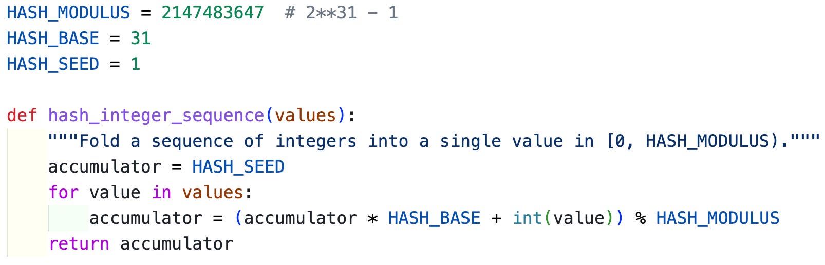
I can cheat and simply not use a proper 32-bit hash. In this case, I choose to use the most boring rolling hash imaginable:

Folded left to right over the sequence, starting from h = 1. Because every accumulator stays below 231-1 (a Mersenne prime), the biggest intermediate you ever form is about 31 * 231 ≈ 236, which is roughly a hundred-thousand times below the 253 , so hopefully we shall stay in the int type territory.9

So, in Python land, this simple hash looks like this:

In APL land that will look quite simple actually (I mean it, prepare yourself for this):

APL’s reduction f/ associates right-to-left, but the recurrence above is a left fold. Reversing the array first resolves this: 1, ⍵ prepends the seed, ⌽ reverses, and folding the reversed array from the right visits the original values in order. For, Hash 1 2 3 the reduction is 3 f (2 f (1 f 1)) where the innermost 1 f 1 is 31×⍵+1, and each outer step multiplies the accumulator (⍵) by 31 and adds the next value (⍺). This is the same recurrence as the Python loop, so the two hashes agree exactly. I checked. So far so easy, now let’s do the thing you’re here for.

Let’s start with reading the file, in python it’s too obvious so I won’t get into it but let me show you the way I’ve done it for APL.

Nah. I’m kidding (although it is correct, just fyi). What I did was simply this:

This defines a function named ReadMatrix. It takes a file path as its input (⍵) and passes a three-item list to the built-in ⎕CSV: the file path, an empty vector (⍬) to use the default comma separator, and 4 to automatically parse and return the data as a simple numeric matrix. See APL is not all that complicated ! Just RTFM !!!

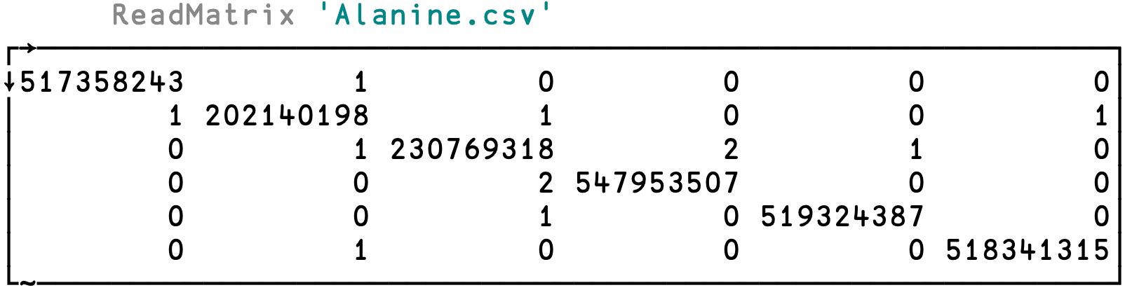
Now that we have our matrix in APL looking something like this:

I think the first step to start off this implementation will be to start by thinking about what the function will look like and I’m thinking of it something like this:

So, let’s start by thinking about how to take these parameters in. For some context, ⍺ and ⍵ represent the left and right arguments of a user-defined function (like a dfn).

In 2 ECFP ‘file.csv’, ⍺ is 2 and ⍵ is ‘file.csv’. Now we also know that I want this default optional flag for useStereo set as 1 (true). Now that I think about it the natural thing to do is also to set 2 as the default radius given the popularity of ECFP_4, so something like ECFP ‘file.csv‘ would work as ECFP_4 with stereochemistry considered. So, I think I can start off with something like this:

ECFP is a dfn so it can close over the constants below. ⍺←2 supplies the default left argument. The left argument may be a scalar radius or a pair (radius useStereo): ⊃⍺ takes the radius, and 2⊃⍺,1 takes the second element if you gave one, otherwise the appended default 1. So (2 0) ECFP file.csv basically ignores any stereochemistry flags.

We take in the file path as the right argument which we represent with ⍵ as I explained before. So, ReadMatrix ⍵ should give us the matrix we need to work with. Once we have that, we have to think about how many rows and columns we have. Recall here that in the format I’ve specified, number of rows could be either same as or one more than the number of columns. This is due to the fact that we may have parity row at the end of the matrix if the molecule has specified stereochemistry.

n is the number of atoms in the given matrix called raw. Number of atoms here is equal to the number of columns in the matrix. The idiomatic way to get the number of rows as I understand it is to use the tally (≢) over the matrix and there could be many ways to get the number of columns like either transposing the matrix and taking the tally of that (≢⍉) or if we know the shape (in our case 2d), we can simply take the second element of the shape like (2⊃⍴). Here I’ve used another option, which is to right reduce the shape of the matrix (⊢/⍴). This approach simply gives the rightmost element in the shape of the matrix which in our case is the column size, but this also generalizes to higher dimensional matrices, but we don’t care about that here.

Now, let’s try to extract the last line iff we have the useStereo flag set to 1 and the number of rows is one more than number of columns. Just for the sake of consistency, we should return parity list of zeros in case there’s no stereochemistry/parity specified or in case useStereo is set to 0. If you read the last paragraph again and read from right to left of the code block [6], I think you’d agree that this is very readable. We take the last row of the matrix using ⊢⌿raw. Remember this could either be parity row or simply a row in the symmetric adjacency matrix. We then multiply this extracted row by the boolean condition ((≢raw)>n). If the matrix has more rows than columns, this evaluates to 1 (true) and leaves the parity data exactly as it was. If the condition evaluates to 0 (false), the multiplication instantly converts the row into our fallback list of zeros. Finally, we multiply this result by the useStereo flag. If stereochemistry is turned off (0), this final multiplication acts as a switch to zero out the array.

We can then extract the top n rows from the raw data to take the square adjacency matrix M, from which the diagonal is extracted to retrieve the initial atomic identifiers ids0 using dyadic transpose.

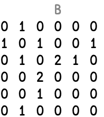
Then diagonal of M is effectively erased to create the bond order matrix B (using an outer product which results in 1 everywhere other than diagonal), which is then converted into a strict boolean adjacency matrix A0 where any existing bond simply becomes a 1.

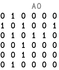
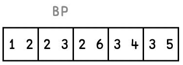
Because this matrix is symmetric, an upper-triangular boolean mask is applied to A0 to ignore redundant mirrored connections, allowing the ⍸ (Where) function to extract the exact (i, j) coordinate pairs for every unique bond into a list BP.

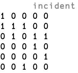
After tallying this list to determine m, the total number of unique bonds, an outer product evaluates whether each atom index is a member of each bond coordinate pair, ultimately generating an n by m incidence matrix that maps exactly which atoms are connected to which bonds. Recall that incident represents an incidence matrix. It is a grid with n rows (representing every atom) and m columns (representing every unique bond).

Now comes the most important piece of the puzzle.

The Step function executes a single iteration of ECFP, updating the state of every atom simultaneously.

First, it unpacks the current state from the right argument ⍵, which includes the iteration counter (t), current identifiers (ids), stereo completion flags (done), topological coverage (cover), and historical accumulators. It then evaluates distinct for each atom (from 1 to n) by finding its neighbors in the bond matrix B and checking if the total number of neighbors equals the number of unique neighbor identifiers. This identifies atoms whose immediate surroundings are perfectly resolved.

Next, it calculates the boolean should array to determine which atoms are ready to incorporate stereochemical parity. An atom qualifies only if stereochemistry is enabled globally, the atom has a non-zero parity value, it hasn’t already been processed (~done), and its neighbors are currently distinct.

The hashing happens in the newids assignment, per atom, individually. For a given atom, it extracts the bond orders and the identifiers of its neighbors, pairing them into a matrix P. To ensure the resulting hash is independent of the input atom order, P is sorted lexicographically (P[⍋P;]) and flattened. This sorted neighbor data is prefixed with the iteration step t and the atom’s current ID. If the should flag is true for this atom, its parity value is appended to the end of the sequence. This canonical sequence is then reduced into a single integer via a Hash function.

Then, the function increases the topological radius of each atom. newcover uses boolean inner product (A0∨.∧cover) against the adjacency matrix to organically “grow” each atom’s known neighborhood outward by one bond. The function ends by returning the updated state bundle for the next step: the incremented iteration t+1, the newly hashed newids, the updated done mask, the expanded newcover, and the respective historical accumulators.

Then, the init array consists of the starting iteration step 1, initial atomic identifiers ids0, an n-length vector of zeros representing the done stereochemistry flags, and an n by m matrix of zeros tracking the initial topological cover. It also initializes the three historical accumulators with matching baseline structures: a copy of ids0 for the identifier history, a zero vector for the iteration history, and a zero matrix for the coverage history.

Next, the power operator (⍣) executes the Step function exactly radius times. It feeds the init bundle into the first iteration, and then iteratively passes the output of each step as the input to the next, saving the ultimate output state in the variable final.

Finally, the diamond separator (⋄) is used to perform multiple assignments on a single line to unpack the results. By using the pick function (⊃), it extracts the 5th, 6th, and 7th elements from the final state array, assigning the accumulated history of identifiers to accID, the iteration steps to accIT, and the topological coverage maps to accCOV.

Now, we need to isolate the definitive list of unique structural features (identifiers), ensuring that redundant topological coverages are discarded in favor of the earliest discovered version.

First, it identifies the baseline “radius-0” features i.e. individual atoms before any radius expansion. It does this by summing the rows of the coverage matrix (accCOV); if a row’s sum is zero, the feature has no bonds and is flagged in the boolean vector empt. The code extracts these specific identifiers from the history (accID) and deduplicates them to form the base list.

Next, it filters out these empty features to focus on the higher-radius structures, generating a list of indices (keep) for everything else. It uses these indices to extract the remaining identifiers into ID2, iteration steps into IT2, and coverage maps into COV2. To ensure deterministic tie-breaking later, it calculates a sorting order (ord) based first on the iteration step (prioritizing features discovered earlier) and secondarily on the identifier value itself. ID2 and COV2 are then reordered using this sorting permutation.

With the data properly ordered, the algorithm eliminates redundant structural representations. It splits the COV2 matrix into a list of row vectors and uses the index function (⍳) to find the first occurrence of each unique topological coverage pattern (first). It then compares this “first occurrence index” against each row’s actual sequential index (⍳≢first). If the indices match, it means this is the first time the algorithm has seen this exact coverage pattern, and it is marked with a 1 in the win boolean mask. If they do not match, the feature is a duplicate and is marked 0.

Finally, we apply the win mask to ID2 to extract only the identifiers of the unique, “winning” features. This list is concatenated with the base list of radius-0 identifiers, deduplicated one last time (∪), sorted into ascending order by the anonymous function {⍵[⍋⍵]}, and returned as the final, canonical list of molecular hashes.

And that’s it ! That’s the implementation of ECFP in APL. Now comes the time to check if this is correct and to do this I’ve implemented the same thing in NumPy and checked and it works!

Read the original source

Lobsters

Publisher

Originally by Manas Mahale

---

0 Comments

Log in to join the conversation.

No comments yet. Be the first to share your thoughts.